Keck-DEIMOS HOWTO
Overview
This doc goes through a full run of PypeIt on a multi-slit observation with Keck/DEIMOS. The following was performed on a Macbook Pro with 8 GB RAM (we recommend 32GB+ for DEIMOS) and took ~45min for the one detector.
Setup
Organize data
Place all of the files in a single folder. Mine is named
/home/xavier/Projects/PypeIt-development-suite/RAW_DATA/keck_deimos/1200G_M_7750
(which I will refer to as RAW_PATH).
The files within this folder are:
$ ls
DE.20170425.09554.fits.gz  DE.20170425.09803.fits.gz  DE.20170425.53065.fits.gz
DE.20170425.09632.fits.gz  DE.20170425.50487.fits.gz
DE.20170425.09722.fits.gz  DE.20170425.51771.fits.gz
It is perfectly fine for the files to contain more than one mask or observations with various gratings. But be sure to include all of the calibrations for each.
Run pypeit_setup
The first script you will run with PypeIt is pypeit_setup, which examines your raw files and generates a sorted list and (when instructed) one PypeIt Reduction File per instrument configuration.
Complete instructions are provided in Setup.
Here is my call for these data:
cd folder_for_reducing   # this is usually *not* the raw data folder
pypeit_setup -r ${RAW_PATH}/DE. -s keck_deimos -c A
This creates a PypeIt Reduction File in the folder named
keck_deimos_A beneath where the script was run.
Note that $RAW_PATH should be the full path, i.e. including a /
at the start.
You will likely see a few WARNINGs about not determining frames of a few types (e.g. align). You may ignore these (and most other) WARNING messages of PypeIt.
If your files included more than one setup (including multiple
masks), then you may wish to replace A in the call to
pypeit_setup with B or some
other setup indicator. Inspect the *.sorted file in the setup_files/
folder to see all the options.
For this example, my .pypeit file in the keck_deimos_A directory looks like this:
# Auto-generated PypeIt input file using PypeIt version: 2.0.0
# UTC 2026-02-10T07:57:06

# User-defined execution parameters
[rdx]
spectrograph = keck_deimos

# Setup
setup read
Setup A: null
amp: '"SINGLE:B"'
binning: 1,1
decker: dra11
dispangle: 7699.95654297
dispname: 1200G
filter1: OG550
setup end

# Data block
data read
 path /path/to/PypeIt-development-suite/RAW_DATA/keck_deimos/1200G_M_7750
                 filename |                 frametype |                 ra |                dec |  target | dispname | decker | binning |          mjd |    airmass | exptime |     dispangle |      amp | filter1 |  lampstat01 |    dateobs |         utc | frameno | calib
DE.20170425.09554.fits.gz |                  arc,tilt |  57.99999999999999 |               45.0 | unknown |    1200G |  dra11 |     1,1 | 57868.110529 | 1.41291034 |     1.0 | 7699.95654297 | SINGLE:B |   OG550 | Kr Xe Ar Ne | 2017-04-25 | 02:39:14.41 |      49 |     0
DE.20170425.09632.fits.gz | pixelflat,illumflat,trace |  57.99999999999999 |               45.0 | unknown |    1200G |  dra11 |     1,1 | 57868.111418 | 1.41291034 |    12.0 | 7699.95654297 | SINGLE:B |   OG550 |          Qz | 2017-04-25 | 02:40:32.06 |      50 |     0
DE.20170425.09722.fits.gz | pixelflat,illumflat,trace |  57.99999999999999 |               45.0 | unknown |    1200G |  dra11 |     1,1 | 57868.112443 | 1.41291034 |    12.0 | 7699.95654297 | SINGLE:B |   OG550 |          Qz | 2017-04-25 | 02:42:02.26 |      51 |     0
DE.20170425.09803.fits.gz | pixelflat,illumflat,trace |  57.99999999999999 |               45.0 | unknown |    1200G |  dra11 |     1,1 | 57868.113392 | 1.41291034 |    12.0 | 7699.95654297 | SINGLE:B |   OG550 |          Qz | 2017-04-25 | 02:43:23.16 |      52 |     0
DE.20170425.50487.fits.gz |                   science | 260.04999999999995 | 57.958444444444446 |   dra11 |    1200G |  dra11 |     1,1 | 57868.584271 |  1.2765523 |  1200.0 | 7699.95654297 | SINGLE:B |   OG550 |         Off | 2017-04-25 | 14:01:27.15 |      85 |     0
DE.20170425.51771.fits.gz |                   science | 260.04999999999995 | 57.958444444444446 |   dra11 |    1200G |  dra11 |     1,1 | 57868.599136 | 1.29137753 |  1200.0 | 7699.95654297 | SINGLE:B |   OG550 |         Off | 2017-04-25 | 14:22:51.01 |      86 |     0
DE.20170425.53065.fits.gz |                   science | 260.04999999999995 | 57.958444444444446 |   dra11 |    1200G |  dra11 |     1,1 |   57868.6141 | 1.31412428 |  1000.0 | 7699.95654297 | SINGLE:B |   OG550 |         Off | 2017-04-25 | 14:44:25.52 |      87 |     0
data end
In this example, all of the frametypes were accurately assigned in the PypeIt Reduction File, so there are no edits to be made. This should generally be the case for DEIMOS. However, if frame types are not assigned correctly, you can edit them following these instructions on the Data Block.
On the other hand, it is the user’s responsibility to remove any bad (or undesired) calibration or science frames from the list. Either delete them altogether or comment out with a #.
Note: we generally recommend to not use bias frames with DEIMOS.
I am going to restrict the reduction to only one of the 8 detectors in the DEIMOS mosaic. Here detector 7, which is one of the middle chips and the redder spectra. I do this by editing the PypeIt file and its parameter block to now read:
# User-defined execution parameters
[rdx]
spectrograph = keck_deimos
detnum = 7
A full run with all 8 detectors (the default) is both long and may tax (or exceed) the RAM of your computer. Therefore, you may wish to reduce 1 or 2 detectors at a time in this fashion. For more than one detector, use a list for detnum (e.g. detnum = 3,7). Also, note that PypeIt can construct image mosaics for detectors separated along the dispersion axis. This is now the default approach for Keck DEIMOS, where a mosaic is constructed for each blue-red detector pair, see here.
Main Run
Once the PypeIt Reduction File is ready, the main call is simply:
cd keck_deimos_A
run_pypeit keck_deimos_A.pypeit -o
The -o indicates that any existing output files should be overwritten. As
there are none, it is superfluous but we recommend (almost) always using it.
The PypeIt’s Core Data Reduction Executable and Workflow doc describes the process in some more detail.
Inspecting Files
As the code runs, a series of files are written to the disk.
Calibrations
The first set are Calibrations. What follows are a series of screen shots and PypeIt QA PNGs produced by PypeIt.
Slit Edges
The code will automatically assign edges to each slit on the detector. This includes using information from the slitmask design recorded in the FITS file, as described in Slitmask ID assignment and missing slits
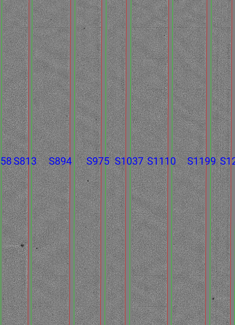
Here is a zoom-in screen shot from the first tab in the ginga window after using the pypeit_chk_edges script, with this explicit call (be patient with ginga):
pypeit_chk_edges Calibrations/Edges_A_1_07.fits.gz
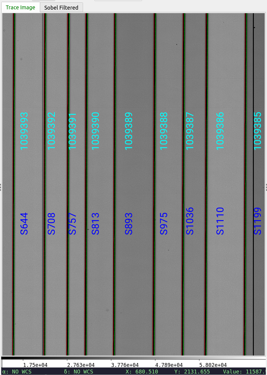
Note the 07 in the filename refers to the detector 7.
The data is the combined flat images and the green/red lines indicate the left/right slit edges (green/magenta in more recent versions). The dark blue labels are the internal slit identifiers of PypeIt. The cyan numbers are the user-assigned ID values of the slits.
See Edges for further details.
Arc
Here is a screen shot of most of the arc image as viewed with ginga:
ginga Calibrations/Arc_A_1_DET07.fits
As typical of most arc images, one sees a series of arc lines, here oriented approximately horizontally.
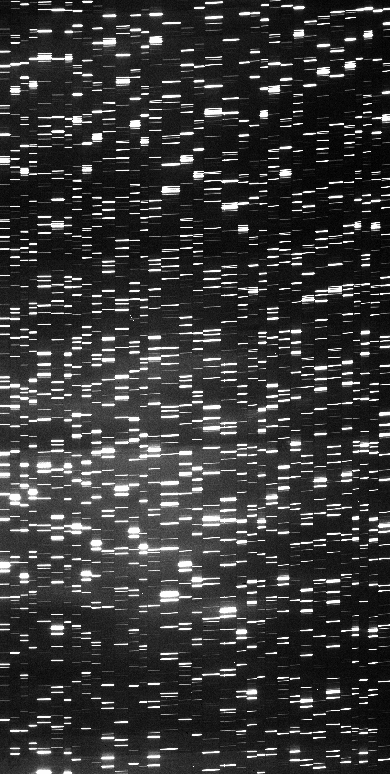
See Arc for further details.
Wavelengths
One should inspect the PypeIt QA for the wavelength calibration. These are PNGs in the QA/PNG/ folder.
Note: there are multiple files generated for every slit.
When the reduction is complete, you may prefer to scan
through them by opening the HTML file under QA/.
1D
Here is an example of the 1D fits, written to
the QA/PNGs/Arc_1dfit_A_1_07_S0758.png file:
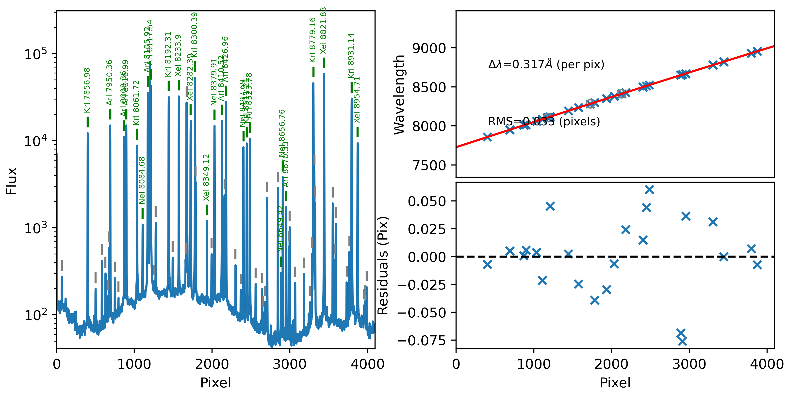
What you hope to see in this QA is:
On the left, many of the blue arc lines marked with green IDs
In the upper right, an RMS < 0.1 pixels
In the lower right, a random scatter about 0 residuals
See WaveCalib for further details.
2D
There are several QA files written for the 2D fits.
Here is QA/PNGs/Arc_tilts_2d_A_1_07_S0758.png:
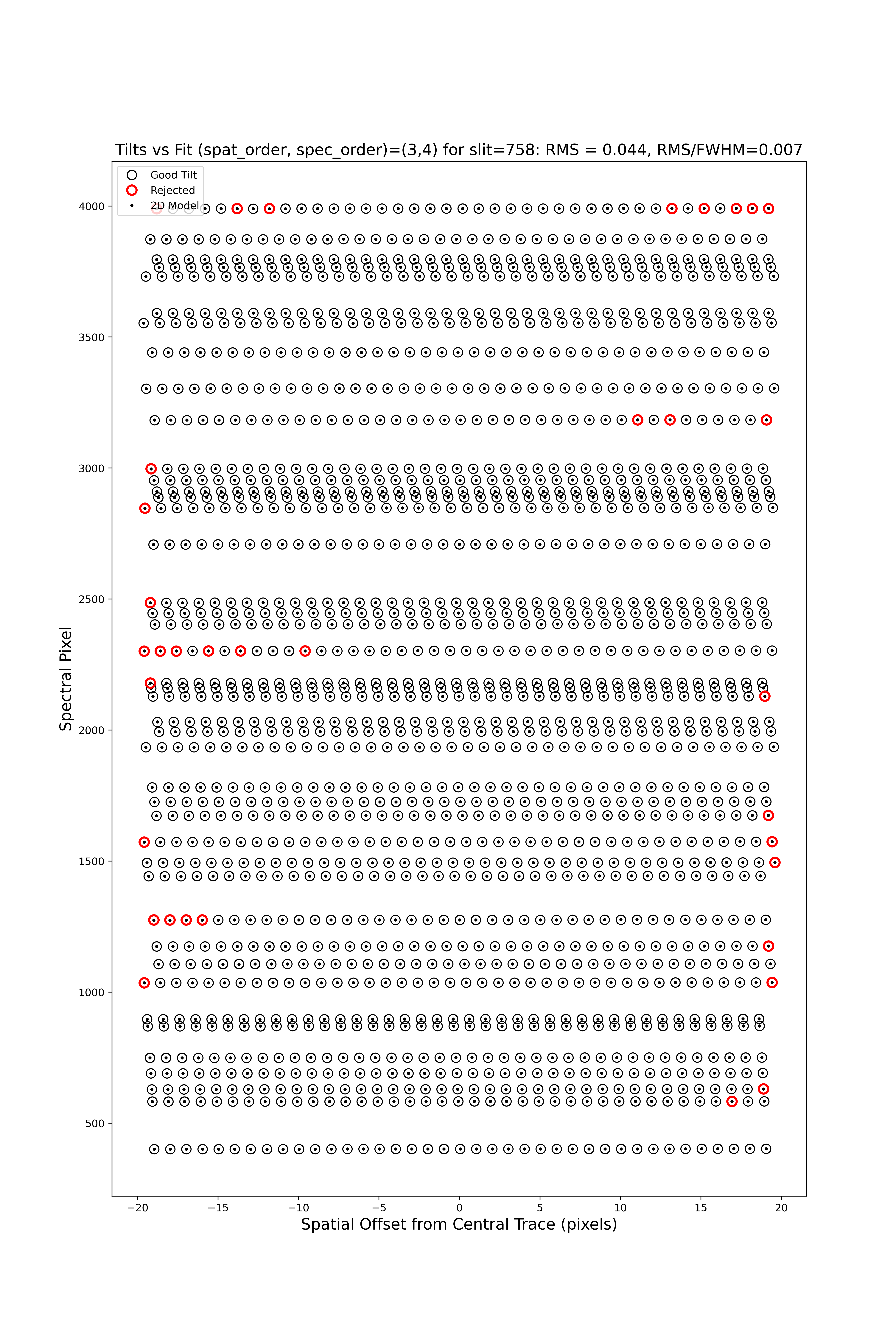
Each horizontal line of circles traces the arc line centroid as a function of spatial position along the slit length. These data are used to fit the tilt in the spectral position. “Good” measurements included in the parametric trace are shown as black points; rejected points are shown in red. Provided most were not rejected, the fit should be good. An RMS<0.1 is also desired.
See WaveCalib for further details.
Flatfield
The code produces flat field images for correcting pixel-to-pixel variations and illumination of the detector.
Here is a zoom-in screen shot from the first tab in the ginga window (pixflat_norm) after using pypeit_chk_flats, with this explicit call:
pypeit_chk_flats Calibrations/Flat_A_1_07.fits
One notes the pixel-to-pixel variations; these are at the percent level. The slit edges defined by the code are also plotted (green/red lines; green/magenta in more recent versions). The regions of the detector beyond the slit boundaries have been set to unit value.
See Flat for further details.
Spectra
Eventually (be patient), the code will start
generating 2D and 1D spectra outputs. One per standard
and science frame, located in the Science/ folder.
Spec2D
Slit inspection
It is frequently useful to view a summary of the slits successfully reduced by PypeIt. The pypeit_parse_slits, with this explicit call:
pypeit_parse_slits Science/spec2d_DE.20170425.50487-dra11_DEIMOS_2017Apr25T140121.014.fits
this prints, detector by detector, the SpatID (internal PypeIt name), MaskID (user ID), and Flags for each slit. Those with None have been successfully reduced.
Visual inspection
Here is a screen shot from the third tab in the ginga window (sky_resid-det07) after using pypeit_show_2dspec, with this explicit call:
pypeit_show_2dspec Science/spec2d_DE.20170425.50487-dra11_DEIMOS_20170425T140121.014.fits --det 7
For DEIMOS masks with many slits, the display time is substantial. You may prefer to limit viewing only a subset of the channels with the –channels option.
The green/red lines are the slit edges (green/magenta in more recent versions). The orange line shows the PypeIt trace of the object and the orange text is the PypeIt assigned name. Yellow lines indicate sources that were auto-magically extracted based on the mask design (i.e. they had insufficient S/N for detection). The night sky and emission lines have been subtracted.
See Spec2D Output for further details.
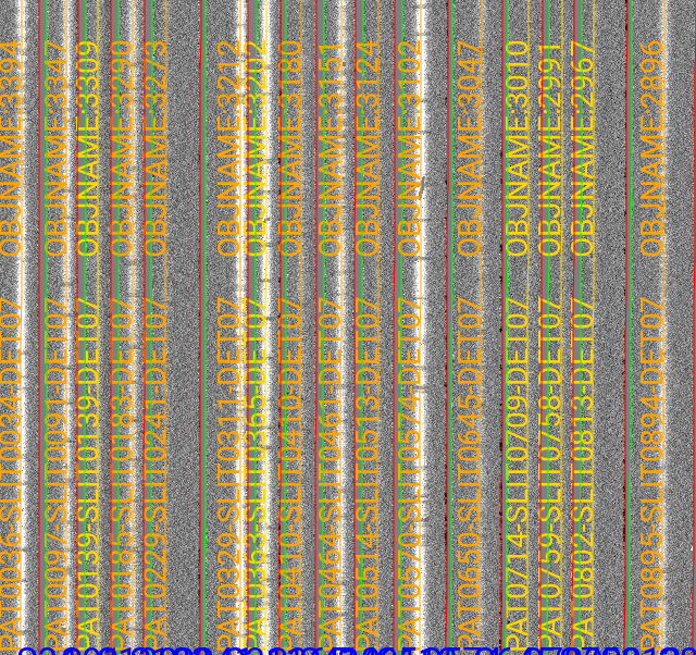
Spec1D
You can see a summary of all the extracted sources in spec1d*.txt
files in the Science/ folder. Here is the top of the one I’ve
produced named spec1d_DE.20170425.50487-dra11_DEIMOS_20170425T140121.014.fits:
| slit |                    name | maskdef_id | objname |     objra |   objdec | spat_pixpos | spat_fracpos | box_width | opt_fwhm |   s2n | maskdef_extract | wv_rms |
|   34 | SPAT0036-SLIT0034-DET07 |    1039404 |    3394 | 260.08018 | 57.96760 |        36.4 |        0.561 |      3.00 |    0.935 | 16.78 |           False |  0.052 |
|   91 | SPAT0097-SLIT0091-DET07 |    1039403 |    3347 | 260.08404 | 57.94896 |        96.9 |        0.630 |      3.00 |    0.868 | 11.74 |           False |  0.041 |
|  139 | SPAT0139-SLIT0139-DET07 |    1039402 |    3309 | 260.08660 | 57.97074 |       138.8 |        0.496 |      3.00 |    0.593 |  2.49 |            True |  0.063 |
|  183 | SPAT0185-SLIT0183-DET07 |    1039401 |    3290 | 260.08949 | 57.94758 |       185.0 |        0.531 |      3.00 |    0.849 | 10.12 |           False |  0.048 |
|  241 | SPAT0229-SLIT0241-DET07 |    1039400 |    3273 | 260.09227 | 57.94045 |       229.5 |        0.284 |      3.00 |    0.802 |  1.73 |           False |  0.032 |
|  311 | SPAT0329-SLIT0311-DET07 |    1039399 |    3212 | 260.09824 | 57.98572 |       329.2 |        0.812 |      3.00 |    0.906 | 17.72 |           False |  0.056 |
The maskdef_id and objname are user supplied in the mask design.
Serendipitous sources will be named SERENDIP. The maskdef_extract flag
indicates whether the extraction was ‘forced’, i.e. the source was not
detected by PypeIt so extraction was performed based on the mask design.
One can generate a similar, smaller set of output using the –list option with pypeit_show_1dspec:
pypeit_show_1dspec Science/spec1d_DE.20170425.50487-dra11_DEIMOS_20170425T140121.014.fits --list
Last, here is a screen shot from the GUI showing the 1D spectrum after using pypeit_show_1dspec, with this explicit call:
pypeit_show_1dspec Science/spec1d_DE.20170425.50487-dra11_DEIMOS_20170425T140121.014.fits --exten 23
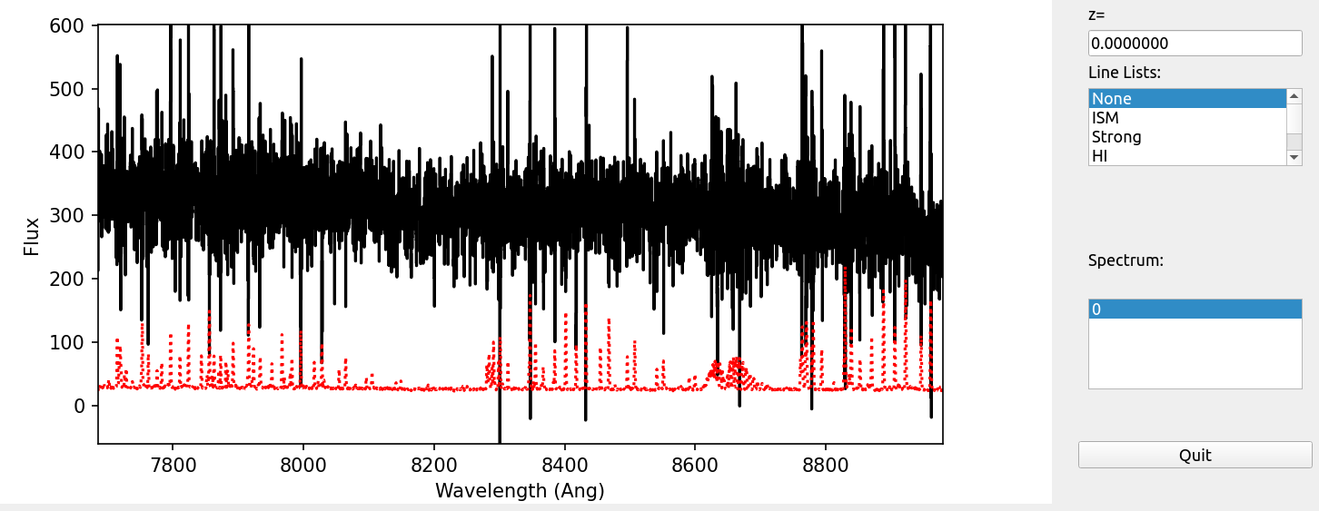
THIS IMAGE IS CURRENTLY OUT OF DATE.
The black line is the flux and the red line is the estimated error.
See Spec1D Output for further details.
Fluxing
The results can be flux calibrated using archived sensitivity functions. To do so first create a
fluxing file, named keck_deimos_1200g_m_7750.flux in this example:
[fluxcalib]
use_archived_sens = True

# User-defined fluxing parameters
flux read
  filename
  Science/spec1d_DE.20170425.50487-dra11_DEIMOS_20170425T140121.014.fits
flux end
Next run the flux calibration tool:
pypeit_flux_calib keck_deimos_1200g_m_7750.flux
The results can be viewed by passing –flux to pypeit_show_1dspec:
pypeit_show_1dspec Science/spec1d_DE.20170425.50487-dra11_DEIMOS_20170425T140121.014.fits --exten 23 --flux
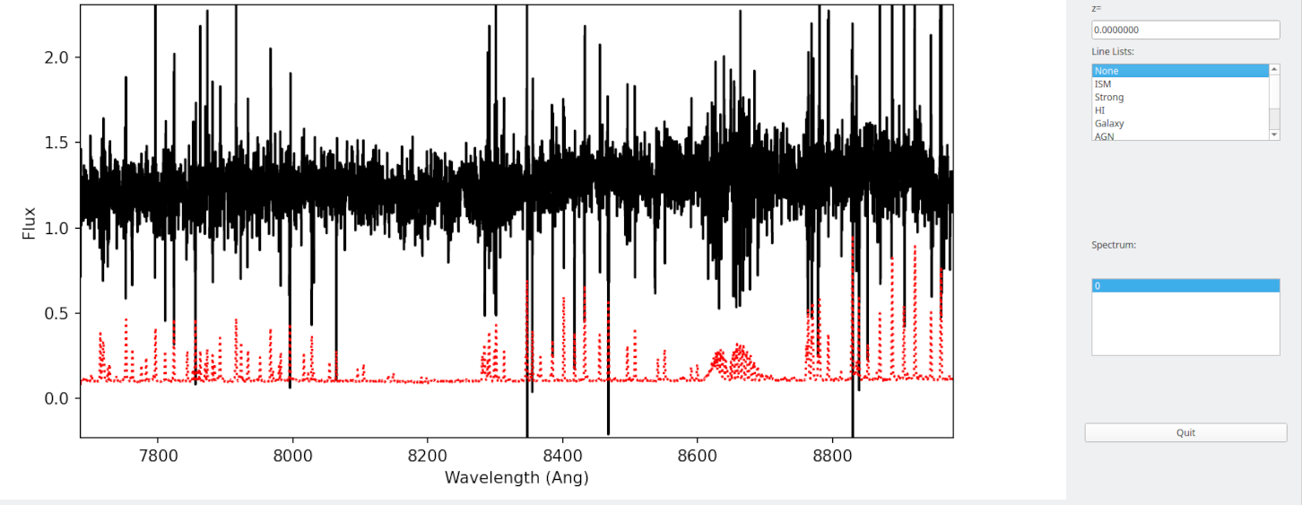
The archived sensitivity functions for DEIMOS are currently experimental and should be used with caution. See Fluxing for more details on flux calibration with PypeIt.
Flexure
The default run performs a flexure correction, slit-by-slit based on analysis of the sky lines to impose a fixed pixel shift for each detector in the spectral dimension. For a more accurate solution, it may be preferred to perform flexure across both detectors.
See pypeit_multislit_flexure for full details on this procedure.