Detector Mosaics
If the geometry of each detector in a detector array is known a priori, PypeIt can construct a mosaic of the detector data for further processing, instead of processing the detector data individually. This is currently the default approach for Gemini/GMOS and Keck/DEIMOS only.
Coordinate Conventions
Coordinate conventions are critical to understanding how PypeIt constructs the detector mosaics. In general, we adopt the standard numpy/matplotlib convention (also identical to how 2D numpy arrays are displayed in ginga), where the first axis is along the ordinate (Cartesian \(y\)) and the second axis is along the abscissa (Cartesian \(x\)). We also assume the pixel coordinates are with respect to the pixel center (i.e., not its bottom-left corner).
For example, to construct arrays with the Cartesian \(x\) and \(y\) pixel coordinates for an image with a specified shape:
import numpy as np
shape = (256, 512)
x, y = np.meshgrid(np.arange(shape[1]), np.arange(shape[0]))
Note that the shape of the image can be interpreted as the number of pixels
along \(y\), then the number of pixels along \(x\) (e.g., (ny,nx)).
You can also construct an array with the vertices of the image extent:
box = np.array([[-0.5,                 -0.5],
                [shape[0]-0.5,         -0.5],
                [shape[0]-0.5, shape[1]-0.5],
                [-0.5,         shape[1]-0.5]])
Note the coordinates are ordered in the same way as the image with Cartesian
\(x\) in box[:,1] and Cartesian \(y\) in box[:,0]. Plotting the
results shows the expected image orientation:
from matplotlib import pyplot

fig = pyplot.figure(figsize=pyplot.figaspect(1/2.))

# Plot the x coordinates
ax = fig.add_subplot(1,2,1)
# Note the limits are set given that the shape provides (ny, nx)
ax.set_xlim([-10, shape[1]+10])
ax.set_ylim([-10, shape[0]+10])
ax.set_xlabel('Cartesian x [pixels]')
ax.set_ylabel('Cartesian y [pixels]')
ax.set_title('x image')
ax.imshow(x, origin='lower', interpolation='nearest')
# Note the array slicing selects x then y
ax.scatter(box[:,1], box[:,0], marker='o', edgecolor='k', s=50, facecolor='none')

# Plot the y coordinates
ax = fig.add_subplot(1,2,2)
ax.set_xlim([-10, shape[1]+10])
ax.set_ylim([-10, shape[0]+10])
ax.set_xlabel('Cartesian x [pixels]')
ax.set_ylabel('Cartesian y [pixels]')
ax.set_title('y image')
ax.imshow(y, origin='lower', interpolation='nearest')
ax.scatter(box[:,1], box[:,0], marker='o', edgecolor='k', s=50, facecolor='none')
pyplot.show()
which should produce the following:
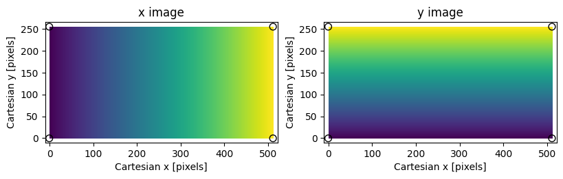
Assumed coordinate system for PypeIt image transformations; small values
are dark, large values are bright. The shape of the image is (256,512).
Black circles mark the vertices of the image bounding box.
Image and Coordinate Transformations
General coordinate transformation matrices are generated using methods in the
transform module, and the image transformations are performed
using scipy.ndimage.affine_transform. For detectors in a mosaic, the key
parameters are the relative offsets between the centers of the detectors and
their rotations about that center. The convenience function used to generate
the transformation matrices is
build_image_mosaic_transform(). Continuing from
the above example, you can can resample the \(x\) coordinate image into a
new image rotated by \(30^\circ\) as follows:
from scipy import ndimage
from pypeit.core import transform
from pypeit.core import mosaic

box = np.array([[-0.5,                 -0.5],
                [shape[0]-0.5,         -0.5],
                [shape[0]-0.5, shape[1]-0.5],
                [-0.5,         shape[1]-0.5],
                [-0.5,                 -0.5]])

# Rotation in degrees
rotation = 30.
# Output image shape
output_shape = (512, 512)
# Shift puts the center of the input image at the center of the output
# image
shift = (output_shape[1]/2 - shape[1]/2, output_shape[0]/2 - shape[0]/2)
# Get the transform
tform = mosaic.build_image_mosaic_transform(shape, shift, rotation=rotation)
# Apply it to the image bounding box
tbox = transform.coordinate_transform_2d(box, tform)
# Use it to resample the input image to the output frame
tx = ndimage.affine_transform(x.astype(float), np.linalg.inv(tform),
                              output_shape=output_shape, cval=np.nan, order=0)
ax = pyplot.subplot()
ax.imshow(tx, origin='lower', interpolation='nearest')
ax.scatter(tbox[:-1,1], tbox[:-1,0], marker='.', color='k', s=50)
ax.plot(tbox[:,1], tbox[:,0], color='k')
ax.set_xlabel('Cartesian x [pixels]')
ax.set_ylabel('Cartesian y [pixels]')
ax.set_title('Rotated by 30 deg')
pyplot.show()
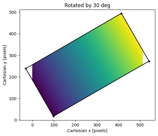
Result of rotating the \(x\)-coordinate image by 30 degrees. Empty
pixels in the transformed image are not shown because they were filled with
np.nan. Note the image regions with pixel coordinates \(<0\) and
\(>511\) are not shown because they are outside the limits of the output
image shape.
Note that we set the output shape of the image directly, but the shape was
insufficient to capture the full size of the rotated image. We avoid this for
the detector mosaics using prepare_mosaic(); see below.
Constructing a Detector Mosaic
To construct a mosaic of the images in a detector array, we need offsets and
rotations for all the relevant detectors. To minimize the interpolation, it is
good practice to set one of the detectors as the reference, which simply means
it has no shift or rotation. All images in a mosaic are currently limited to
having exactly the same shape, and all PypeIt mosaics are created using
nearest-grid-point interpolation (order=0 in
scipy.ndimage.affine_transform) by default (cf., the approach used for
Keck DEIMOS).
Image mosaics in PypeIt are constructed after the Basic Image Processing, meaning that the images to be included in the mosaic obey the PypeIt convention of spectral pixels along the first axis and spatial pixels along the second axis; i.e., the shape of each image is \((N_{\rm spec}, N_{\rm spat})\). Following the conventions above, that means the shifts and rotations should be defined adopting the spatial axis as the Cartesian \(x\) axis and the spectral axis as the Cartesian \(y\) axis. Specifically,
Shifts: Image shifts are defined in unbinned pixels. The first element in the two-tuple should be the spatial shift, and the second is the spectral shift.
Rotations: Rotations are defined in counter-clockwise degrees.
Any affects of the binning on the transformation matrices calculated using the
above inputs are determined by
build_image_mosaic_transform().
For example, the code below places the coordinate images created above in a 3-detector mosaic, with the detectors separated along the dispersion axis.
# Define the shifts and rotations.  Note the shifts are always in the
# dispersion direction.
shift = [(0, -320.), (0., 0.), (0., 320)]
rotation = [-10., 0., 10.]

# Construct the tranformation matrix for each image.
nimg = 3
tforms = [None]*nimg
for i in range(nimg):
    tforms[i] = mosaic.build_image_mosaic_transform(shape, shift[i], rotation=rotation[i])

# Construct the mosaic
msc, _, _, _tforms = mosaic.build_image_mosaic([y.astype(float), x.astype(float),
                                                x.astype(float)], tforms, cval=np.nan)

# Show the result
ax = pyplot.subplot()
ax.set_xlabel('Spatial Position [pixels]')
ax.set_ylabel('Spectral Position [pixels]')
ax.set_title('Detector Mosaic')
ax.set_xlim(-50, msc.shape[1]+50)
ax.set_ylim(-50, msc.shape[0]+50)
ax.imshow(msc, origin='lower', interpolation='nearest')
color = ['C1', 'C3', 'C4']
for i in range(nimg):
    tbox = transform.coordinate_transform_2d(box, _tforms[i])
    ax.scatter(tbox[:-1,1], tbox[:-1,0], marker='.', color=color[i], s=50)
    ax.plot(tbox[:,1], tbox[:,0], color=color[i], lw=2)
pyplot.show()
In the previous section we set the shape of the transformed image directly, and
the result was that the shape was to small to capture the full rotated image.
Here, because no output shape is passed, the call to
build_image_mosaic() uses
prepare_mosaic() to determine the shape required to
capture the full mosaic and adjust the transformation matrices from a relative
to absolute frame. These adjusted transformations are returned by
build_image_mosaic() and can be applied to additional
images or, as in the example above, the vertices of the input images to show the
bounding boxes of the input images in the output mosaic.
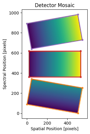
Mock mosaic with three detectors offset in the spectral (dispersion)
direction. Orange, red, and purple boxes are the bounding boxes for the 1st,
2nd, and 3rd input images, respectively. Note that, because we’ve filled the
empty pixels with np.nan values, the unfilled regions in the msc
array are not shown by matplotlib.