PypeIt QA

As part of the standard reduction, PypeIt generates a series of fixed-format Quality Assurance (QA) figures. This document describes the typical outputs, in the typical order that they appear.

This page is still a work in progress.

The basic arrangement is that individual PNG files are created and then a set of HTML files are generated to organize viewing of the PNGs.

HTML

When the code completes (or crashes out), an HTML file is generated in the QA/ folder, one per setup that has been reduced (typically one). An example filename is MF_A.html. These HTML files are out of date, so you’re better off opening the PNG files in the PNGs directory directly.

Calibration QA

The first QA PNG files generated are related to calibration processing. There is a unique one generated for each setup and detector and (possibly) calibration set.

Generally, the title describes the type of QA plotted.

Echelle Order Prediction

When reducing echelle observations and inserting missing orders, a QA plot is produced to assess the success of the predicted locations. The example below is for Keck/HIRES.

Example QA plot showing the measured order spatial widths (blue) and gaps (green) in pixels. The widths should be nearly constant as a function of position, whereas the gaps should change monotonically with spatial pixel.

In the figure above, measured values that are included in the polynomial fit are shown as filled points. The colored lines show the best fit polynomial model used for the predicted order locations. The fit allows for an iterative rejection of points; measured widths and gaps that are rejected during the fit are shown as orange and purple crosses, respectively. The measurements that are rejected during the fit are not necessarily removed as invalid traces, but the code allows you to identify outlier traces that will be removed. None of the traces in the example image above are identified as outliers; if they exist, they will be plotted as orange and purple triangles for widths and gaps, respectively. Missing orders that will be added are included as open squares; gaps are green, widths are blue. To deal with overlap, “bracketing” orders are added for the overlap calculation but are removed in the final set of traces; the title of the plot indicates if bracketing orders are included and the vertical dashed lines shows the edges of the detector/mosaic.

Wavelength Fit QA

PypeIt produces plots like the one below showing the result of the wavelength calibration.

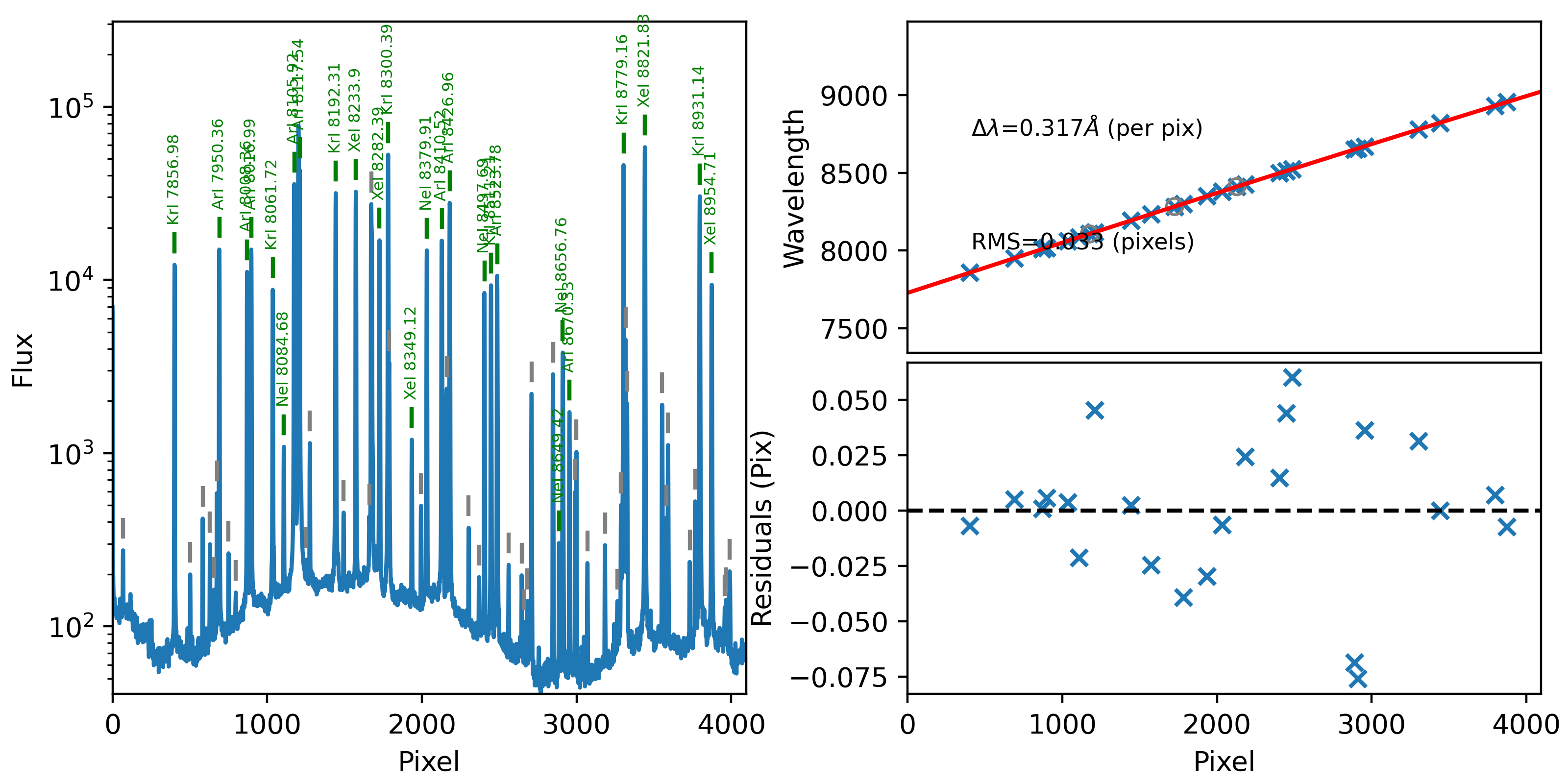
An example QA plot for Keck/DEIMOS wavelength calibration. The extracted arc spectrum is shown to the left with arc lines used for the wavelength solution marked in green. The upper-right plot shows the best-fit calibration between pixel number and wavelength, and the bottom-right plot shows the residuals as a function of pixel number.

See WaveCalib for more discussion of this QA.

Wavelength Tilts QA

PypeIt produces plots like the one below showing the result of tracing the tilts in the wavelength as a function of spatial position within the slits.

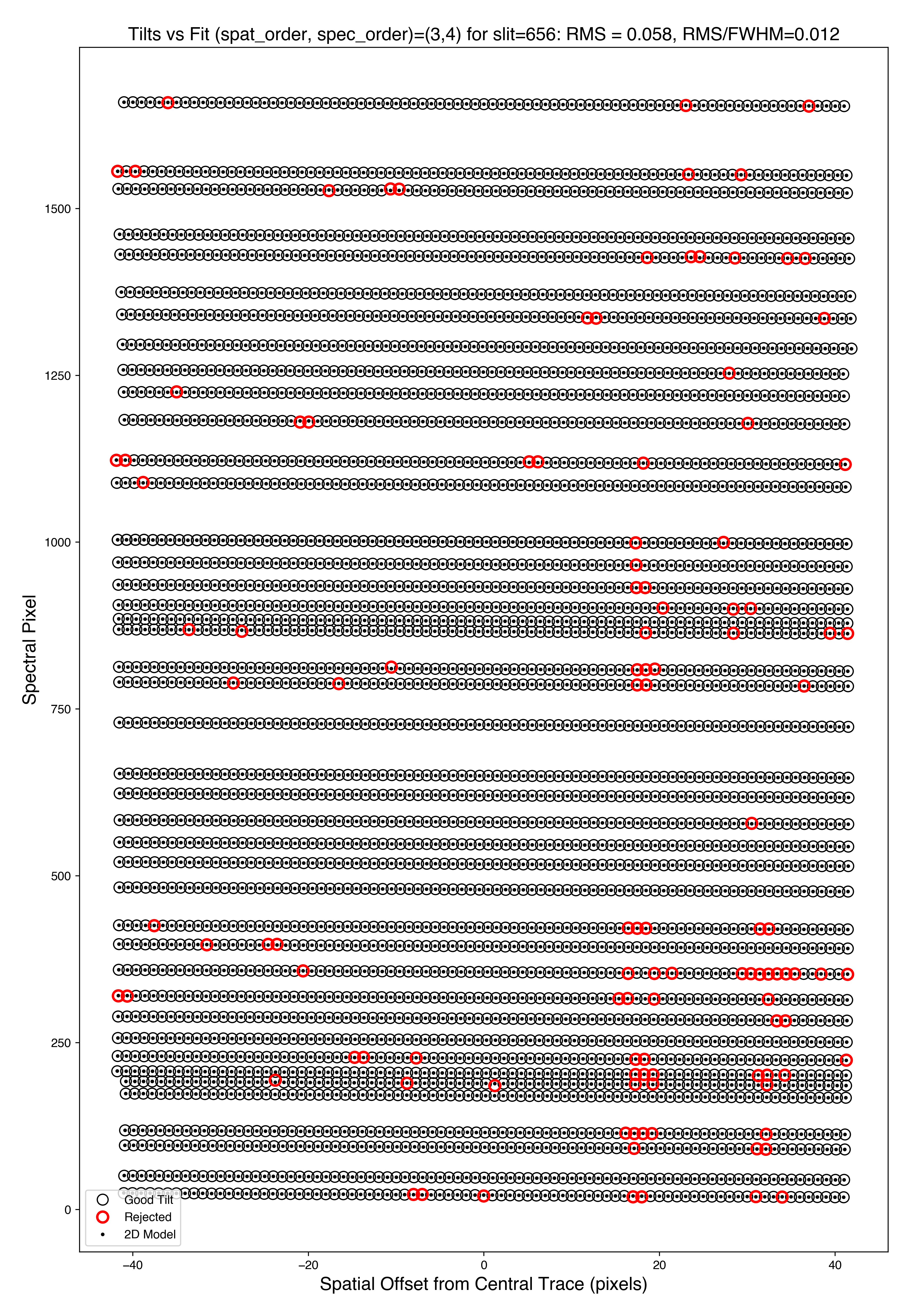
An example QA plot for a single slit in a Keck/MOSFIRE tilt QA plot. Each horizontal line of black dots is an OH line. Red points were rejected in the 2D fitting. Provided most were not rejected, the fit should be good.

See Tilts for more discussion of this QA.

Exposure QA

For each processed, science exposure there are a series of PNGs generated, per detector and (sometimes) per slit.

Spatial Flexure QA

If a spatial flexure correction was performed, the result of the correction is shown in a plot like the one below. The plot shows a few snippets of the science/standard spectral image with overlaid the slit edges as traced in the trace image (dashed lines) and after applying the spatial flexure correction (solid lines). The value of the shift is also reported on the top of the plot.

Spectral Flexure QA

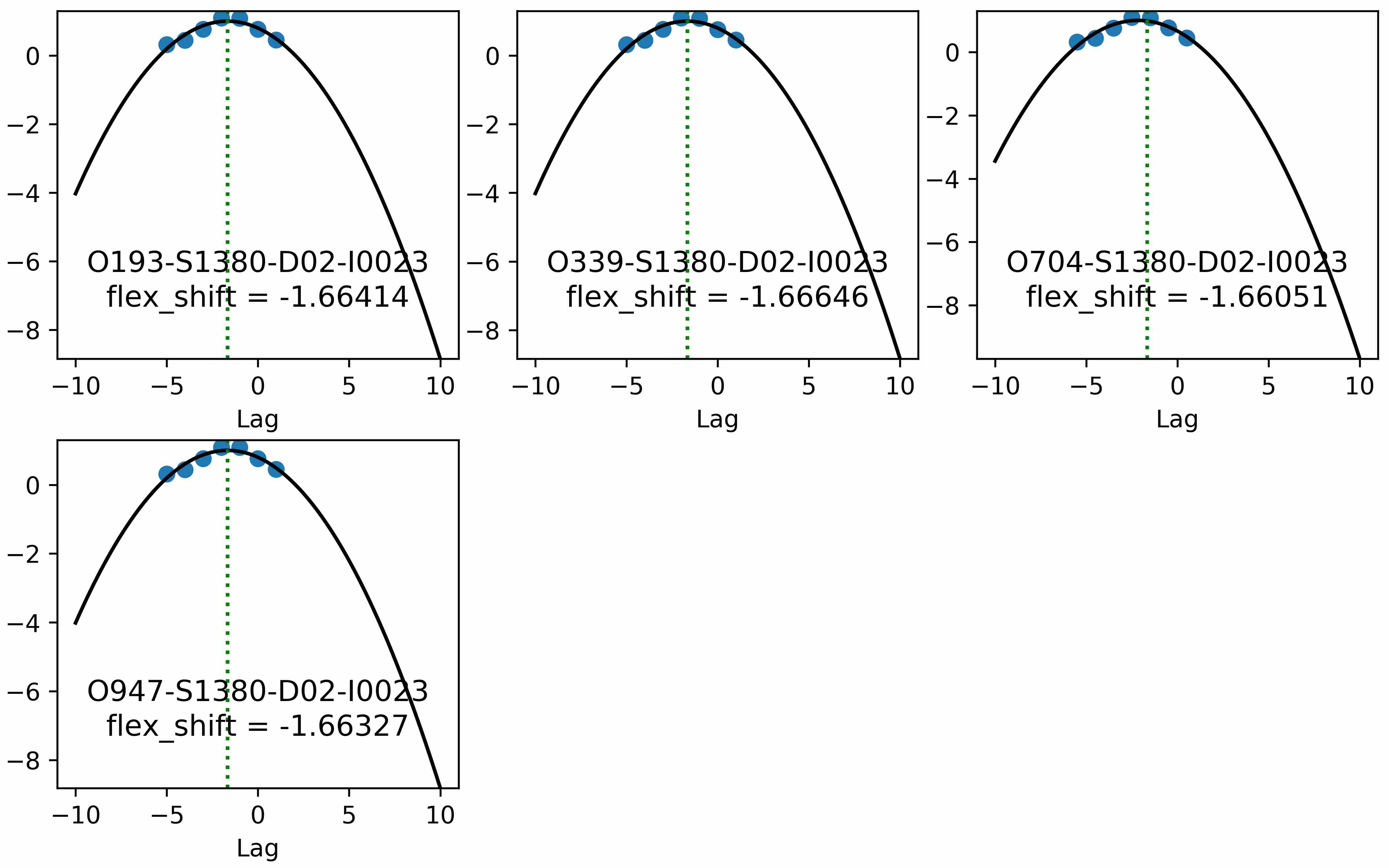
If a spectral flexure correction was performed (default), the fit to the correlation lags per object is shown and the adopted shift is listed. Here is an example:

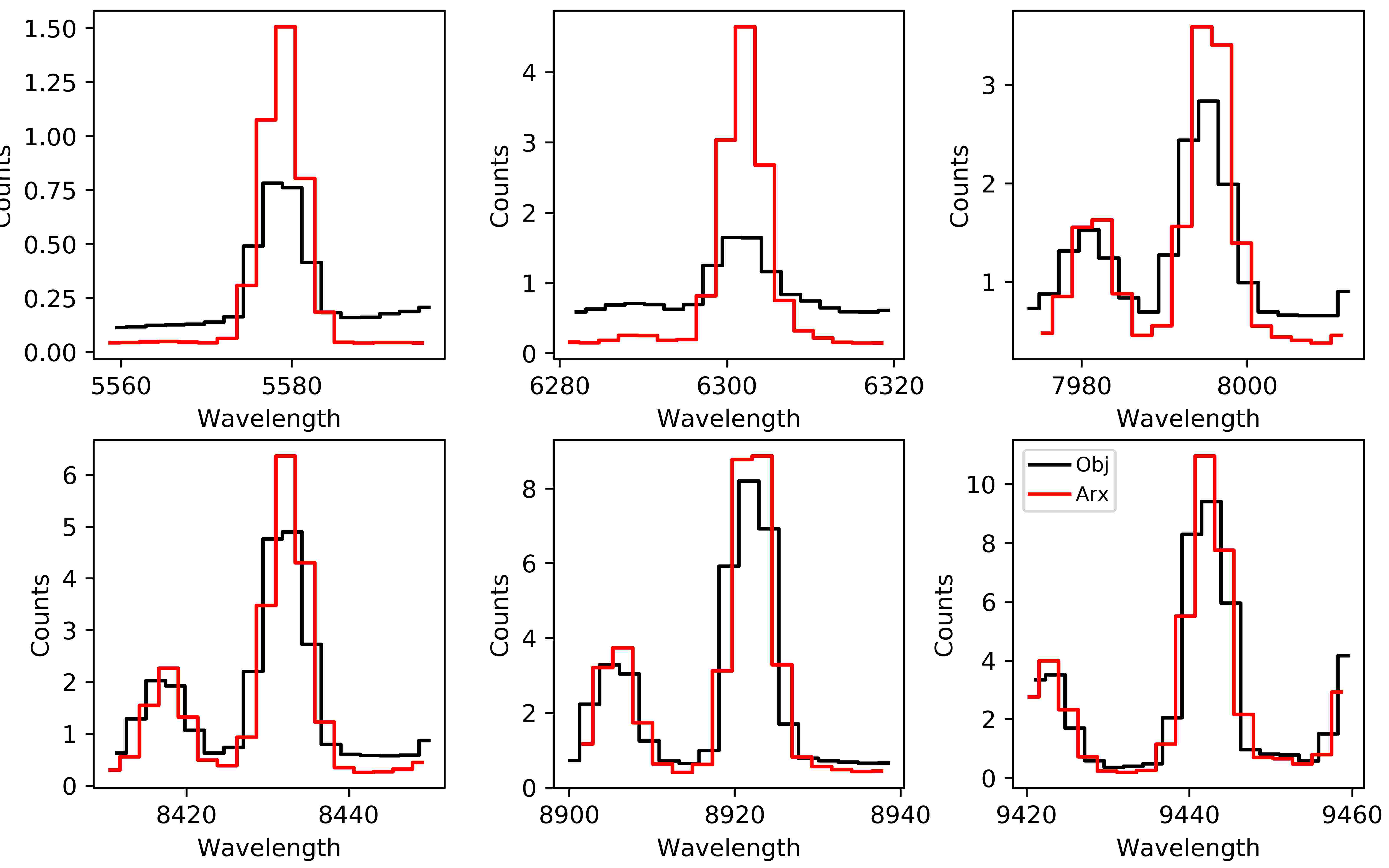
There is then a plot showing several sky lines for the analysis of a single object (brightest) from the data compared against an archived sky spectrum. These should coincide well in wavelength. Here is an example:

Object Finding QA

The object-finding step can be evaluated using the *_obj_prof.png QA files produced during the main PypeIt run. Following the algorithm outlined in Object Finding, the plot provides a visual confirmation of the steps taken to identify the objects in each spec2d frame. The heart of the QA plot is the FWHM-convolved plot of the spectrally-squashed spectral image. Identified objects are marked with green or yellow circles to indicate objects that exceed the minimum detection signal-to-noise ratio (SNR; red dashed line). Objects in excess of the maximum allowed per slit are in yellow, sorted by SNR.

Examples of object-finding QA files for different types of frames are shown below.

Keck/LRIS Standard Star Frame

Example object finding QA plot for Keck/LRIS, using the long_400_8500_d560 dataset from the PypeIt Development Suite. A total of 6 objects were found whose collapsed SNR exceeded the threshold (\(10\sigma\)), but for only the brightest 5 were marked as “good”, since this is a standard frame and maxnumber_std = 5.

Subaru/FOCAS Faint Object Frame

This shows the spatial profile of the object’s S/N collapsed along the spectral direction. The dashed red line is the S/N threshold set by the FindObjPar Keywords, and the green circle marks the spatial position of the detected object. This plot is useful to assess if the object was correctly detected and if the S/N threshold (snr_thresh) set is appropriate for the observation. You will note that there were 3 objects rejected because we restricted the code to find only 2 objects in the science frame. See Object Finding for further details.

Gemini/GMOS Science Frame

Examples of object finding on three separate slits from a single Gemini/GMOS frame from the GS_HAM_B480_550 dataset in the PypeIt Development Suite. Note that only one of the slits had an object meet the detection threshold specified by instrument parameters.

Object Tracing QA

The object-tracing step can be evaluated using the *_obj_trace.png QA files produced during the main PypeIt run. These plots indicate the extracted spatial peak of the object trace (ordinate) as a function of spectral pixel (abscissa). The value of these plots lies in identifying when the tracing algorithm has gone off the rails and is following something other than the desired spectral object.

Examples of object-tracing QA files for different types of frames are shown below.

Keck/LRIS Standard Star Frame

Example object tracing QA plot for Keck/LRIS, using the long_400_8500_d560 dataset from the PypeIt Development Suite. A total of 6 objects were found whose collapsed SNR exceeded the threshold (\(10\sigma\)), but for only the brightest 5 were marked as “good”, since this is a standard frame and maxnumber_std = 5.

Gemini/GMOS Science Frame

Example object tracing QA plot for Gemini/GMOS, using the GS_HAM_B480_550 dataset from the PypeIt Development Suite. Of the three slits shown above in the Object Fining QA plot, only one had an object found using the criteria specified in the PypeIt Reduction File.

Using the Object Tracing QA Plot for Troubleshooting

The value in these plots lies in troubleshooting when object tracing goes wrong. In the example below, an object was observed using a 150 l/mm grating on the LDT/DeVeny spectrograph at an elevation of 11\(^\circ\) above the horizon (airmass 5). As a result of significant atmospheric dispersion, the point-like object was smeared out into a rainbow and the spectrum appears curved with respect to the slit edges. Using standard PypeIt tracing parameters for this spectrograph, the resulting object trace is shown below.

Attempt at object tracing using standard PypeIt parameters.

Note that the fitted object trace is not monotonic, and jumps at low spectral pixel number (short wavelength) away from the solid trend of the trace toward noise in the image closer to the input trace value. Comparison of this trace with the spec2d image indicates that the tracing did not follow the actual peak in the spectral image. While occasional grey dots indicating “Centroid masked, fit” (as in the Keck/LRIS plots above) are acceptable, contiguous sections (as seen here) are problematic. See Object Tracing for details about parameter changes that can be applied to fix these traces.