Keck/NIRES HOWTO
Overview
This doc goes through a full run of PypeIt on one of our example Keck/NIRES
datasets (specifically the ABBA_wstandard dataset). If you’re having
trouble reducing your data, we encourage you to try going through this tutorial
using this example dataset first. See here to find the
example dataset, please join our PypeIt Users Slack using this invitation link to
ask for help, and/or Submit an issue to Github if you find a bug!
Setup
Before reducing your data with PypeIt, you first have to prepare a PypeIt Reduction File by running pypeit_setup:
pypeit_setup -r $HOME/Work/packages/PypeIt-development-suite/RAW_DATA/keck_nires/ABBA_wstandard/ -s keck_nires -b -c A
where the -r argument should be replaced by your local directory and the
-b indicates that the data uses background images and should include the
calib, comb_id, bkg_id in the pypeit file. This directory only has
one instrument configuration (NIRES only has one configuration anyway), so
setting -c A and -c all is equivalent.
This will make a directory called keck_nires_A that holds a pypeit file
called keck_nires_A.pypeit that looks like this:
# Auto-generated PypeIt input file using PypeIt version: 2.0.0
# UTC 2026-02-10T07:57:06

# User-defined execution parameters
[rdx]
spectrograph = keck_nires

# Setup
setup read
Setup A: null
dispname: spec
setup end

# Data block
data read
 path /path/to/PypeIt-development-suite/RAW_DATA/keck_nires/ABBA_wstandard
         filename |        frametype |               ra |              dec |     target | dispname |    decker | binning |              mjd |          airmass | exptime | dithpat | dithpos | dithoff | frameno | calib | comb_id | bkg_id
s190519_0059.fits | arc,science,tilt | 194.259151362434 | 22.0313494322493 |      GD153 |     spec | 0.55 slit |     1,1 | 58622.3598610573 | 1.03675819208546 |   200.0 |    ABBA |       A |     2.0 |      59 |     0 |       1 |      2
s190519_0060.fits | arc,science,tilt | 194.260349844733 | 22.0313316699865 |      GD153 |     spec | 0.55 slit |     1,1 |  58622.362605849 | 1.04142552296712 |   200.0 |    ABBA |       B |    -2.0 |      60 |     0 |       2 |      1
s190519_0067.fits | arc,science,tilt | 222.661173514297 | 33.0367669564831 | J1450+3302 |     spec | 0.55 slit |     1,1 | 58622.4110204323 | 1.03169892034606 |   300.0 |  MANUAL |    None |     0.0 |      67 |     1 |       3 |     -1
s190519_0068.fits | arc,science,tilt | 222.660207102656 | 33.0382234687118 | J1450+3302 |     spec | 0.55 slit |     1,1 | 58622.4152114045 | 1.03446078772601 |   300.0 |  MANUAL |    None |     0.0 |      68 |     1 |       4 |     -1
s190519_0011.fits |     lampoffflats |             58.0 |             45.0 | DOME PHLAT |     spec | 0.55 slit |     1,1 | 58622.0756482101 | 1.41291034446565 |   100.0 |    none |    None |     0.0 |      11 |   all |      -1 |     -1
s190519_0013.fits |     lampoffflats |             58.0 |             45.0 | DOME PHLAT |     spec | 0.55 slit |     1,1 | 58622.0783221684 | 1.41291034446565 |   100.0 |    none |    None |     0.0 |      13 |   all |      -1 |     -1
s190519_0015.fits |     lampoffflats |             58.0 |             45.0 | DOME PHLAT |     spec | 0.55 slit |     1,1 | 58622.0809961267 | 1.41291034446565 |   100.0 |    none |    None |     0.0 |      15 |   all |      -1 |     -1
s190519_0010.fits |  pixelflat,trace |             58.0 |             45.0 | DOME PHLAT |     spec | 0.55 slit |     1,1 | 58622.0743023767 | 1.41291034446565 |   100.0 |    none |    None |     0.0 |      10 |   all |      -1 |     -1
s190519_0012.fits |  pixelflat,trace |             58.0 |             45.0 | DOME PHLAT |     spec | 0.55 slit |     1,1 | 58622.0769763351 | 1.41291034446565 |   100.0 |    none |    None |     0.0 |      12 |   all |      -1 |     -1
s190519_0014.fits |  pixelflat,trace |             58.0 |             45.0 | DOME PHLAT |     spec | 0.55 slit |     1,1 | 58622.0796502934 | 1.41291034446565 |   100.0 |    none |    None |     0.0 |      14 |   all |      -1 |     -1
data end
For this example dataset, the details of the default pypeit file are not completely correct; see here for an example where the frame typing and dither pattern determinations are correct by default.
The issue with this dataset is that only two pointings in the ABBA pattern for
the standard star observations are available, the exposure time of the standard
observations is longer than expected (and PypeIt set it as science frame),
and the dither pattern of the science frames are set to MANUAL.
PypeIt attempts to assign comb_id and bkg_id to the two standard star
pointings, however, you need to edit the pypeit file to
correct the other errors. The corrections needed are:
Set the frametypes for
s190519_0059.fitsands190519_0060.fitstostandard.Assign the same calibration group to the standard and science frames (i.e., same
calibvalue).Set the
bkg_idfor thescienceframes; see below and A-B image differencing.
The corrected version looks like this (pulled directly from the PypeIt Development Suite):
# Auto-generated PypeIt input file using PypeIt version: 1.12.2.dev118+g6905096d0
# UTC 2023-03-25T04:05:16.591

# User-defined execution parameters
[rdx]
    spectrograph = keck_nires
[reduce]
    [[findobj]]
        snr_thresh = 5
        maxnumber_std = 2

# Setup
setup read
Setup A:
  dispname: spec
setup end

# Data block
data read
 path /Users/dpelliccia/Pypeit/PypeIt-development-suite/RAW_DATA/keck_nires/ABBA_wstandard
         filename |        frametype |               ra |              dec |     target | dispname |    decker | binning |              mjd |          airmass | exptime | dithpat | dithpos | dithoff | frameno | calib | comb_id | bkg_id
s190519_0059.fits |         standard | 194.259151362434 | 22.0313494322493 |      GD153 |     spec | 0.55 slit |     1,1 | 58622.3598610573 | 1.03675819208546 |   200.0 |    ABBA |       A |     2.0 |      59 |     0 |       1 |      2
s190519_0060.fits |         standard | 194.260349844733 | 22.0313316699865 |      GD153 |     spec | 0.55 slit |     1,1 |  58622.362605849 | 1.04142552296712 |   200.0 |    ABBA |       B |    -2.0 |      60 |     0 |       2 |      1
s190519_0067.fits | arc,science,tilt | 222.661173514297 | 33.0367669564831 | J1450+3302 |     spec | 0.55 slit |     1,1 | 58622.4110204323 | 1.03169892034606 |   300.0 |  MANUAL |    None |     0.0 |      67 |     0 |       3 |      4
s190519_0068.fits | arc,science,tilt | 222.660207102656 | 33.0382234687118 | J1450+3302 |     spec | 0.55 slit |     1,1 | 58622.4152114045 | 1.03446078772601 |   300.0 |  MANUAL |    None |     0.0 |      68 |     0 |       4 |      3
s190519_0011.fits |     lampoffflats |             58.0 |             45.0 | DOME PHLAT |     spec | 0.55 slit |     1,1 | 58622.0756482101 | 1.41291034446565 |   100.0 |    none |    None |     0.0 |      11 |   all |      -1 |     -1
s190519_0013.fits |     lampoffflats |             58.0 |             45.0 | DOME PHLAT |     spec | 0.55 slit |     1,1 | 58622.0783221684 | 1.41291034446565 |   100.0 |    none |    None |     0.0 |      13 |   all |      -1 |     -1
s190519_0015.fits |     lampoffflats |             58.0 |             45.0 | DOME PHLAT |     spec | 0.55 slit |     1,1 | 58622.0809961267 | 1.41291034446565 |   100.0 |    none |    None |     0.0 |      15 |   all |      -1 |     -1
s190519_0010.fits |  pixelflat,trace |             58.0 |             45.0 | DOME PHLAT |     spec | 0.55 slit |     1,1 | 58622.0743023767 | 1.41291034446565 |   100.0 |    none |    None |     0.0 |      10 |   all |      -1 |     -1
s190519_0012.fits |  pixelflat,trace |             58.0 |             45.0 | DOME PHLAT |     spec | 0.55 slit |     1,1 | 58622.0769763351 | 1.41291034446565 |   100.0 |    none |    None |     0.0 |      12 |   all |      -1 |     -1
s190519_0014.fits |  pixelflat,trace |             58.0 |             45.0 | DOME PHLAT |     spec | 0.55 slit |     1,1 | 58622.0796502934 | 1.41291034446565 |   100.0 |    none |    None |     0.0 |      14 |   all |      -1 |     -1
data end
Use of the standard frame
By setting the science frames to also be arc and tilt
frames, we’re indicating that the OH sky lines should be used to perform the
wavelength calibration. Generally the standard star observations are not
sufficiently long to have good signal in the sky lines to perform the
wavelength calibration. This is why, generally, we do not
set the standard frames to be also arc and tilt frames, but we use
the wavelength calibration obtained from the science frame (this is why we
give to the standard frames the same calib value as the science frames).
We note, however, that in this specific case the observations of the standard star
are sufficiently long to allow for good signal in the sky lines. Therefore, if
desired, you could set the standard frames to be also arc and tilt frames.
The main data-reduction script (run_pypeit) does not perform the telluric correction; this is done by a separate script. Even if you don’t intend to telluric-correct or flux-calibrate your data, it’s useful to include the standard star observations along with the reductions of your main science target, particularly if the science target is faint. If your object is faint, tracing the object spectrum for extraction can be difficult using only the signal from the source itself. PypeIt will resort to a “tracing crutch” if the source signal becomes too weak. Without the bright standard star trace, the tracing crutch used is the slit/order edge, which will not include the effects of differential atmospheric refraction on the object centroid and therefore yield a poorer spectral extraction.
Dither sequence
In this example dataset, the science object and the standard star are both only
observed at two offset positions. Although PypeIt is able to correctly assign
comb_id and bkg_id for the standard frames (by using the information
on the dither pattern and dither offset), the same is not possible for the
science frames, for which a “MANUAL” dither pattern was used.
We, therefore, edit the PypeIt Reduction File (see the
corrected version above) to assign comb_id and bkg_id to the science frames
as described by A-B image differencing (specifically, see
Image Differencing).
By setting comb_id=3 and bkg_id=4 for frame s190519_0067.fits, we
are indicating that this frame should be treated as frame A and that frame
B should be used as its background. We reverse the values of comb_id
and bkg_id for frame s190519_0068.fits, which indicates that this frame
should be treated as frame B and that frame A should be used as its
background. I.e., the comb_id column effectively sets the numeric identity
of each frame, and the bkg_id column selects the numeric identity of the
frame that should be used as the background image.
When PypeIt reduces the frames in this example, it constructs two images, A-B and B-A, such that the positive residuals in each image are the observed source flux for that observation, which can be combined using 2D coadding.
The use of the comb_id and bkg_id integers is very flexible, allowing
for many, more complicated dithering scenarios; see A-B image differencing.
Core Processing
To perform the core processing of the NIRES data, use run_pypeit:
run_pypeit keck_nires_A.pypeit
The code will run uninterrupted until the basic data-reduction procedures (wavelength calibration, field flattening, object finding, sky subtraction, and spectral extraction) are complete; see PypeIt’s Core Data Reduction Executable and Workflow. Processing of this example dataset takes roughly 10 minutes (on a 2020 MacBook Pro with 16 GB of RAM and a 2GHz i5 processor).
As the code processes your data, it will produce a number of files and QA plots for you to inspect:
Order Edges
The code first uses the trace frames to find the order edges. NIRES is a
fixed-format echelle, meaning that the trace results should always look the
same. To show the results of the trace, run, e.g.:
pypeit_chk_edges Calibrations/Edges_A_7_DET01.fits.gz
which will show the image and overlay the traces (green is the left edge; magenta is the right edge); this should open a ginga window for you if one is not open already. Here is the result from this example dataset:
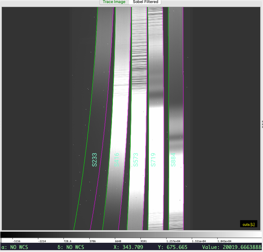
An important check is to ensure that the code has correctly traced the bluest (left-most) order. PypeIt currently expects to find all 5 orders and will fault if it does not.
Tip
If PypeIt faults because it did not find all 5 orders, try adjusting the
edge_thresh parameter; see the User-level Parameters and specifically the
EdgeTracePar Keywords.
Wavelength Calibration
Next the code performs the wavelength calibration. Via the PypeIt Reduction File, we designated two sets of wavelength calibration frames, one for the standard star and one for the science frame. You should inspect the results for both.
First, it’s important to understand PypeIt’s Calibration Frame Naming convention,
specifically the calibration group bit identities used in the output file names.
In this example, two Arc files are produced:
Calibrations/Arc_A_2_DET01.fits and Calibrations/Arc_A_4_DET01.fits.
The 2 and 4 are the bits associated with the calibration group and link
back to which files are associated with each frame type. The
“.calib” File provides the direct association of input frame
with output calibration file.
Combined Arc Frame
You can view the combined arc frame used for, e.g., the standard star observations with ginga:
ginga Calibrations/sArc_A_2_DET01.fits
1D Wavelength Solution
More importantly, you should check the result of the wavelength calibration using the automatically generated QA file; see Wavelength Fit QA. Below is the wavelength-calibration QA plot for the reddest order (order=3). The RMS of the wavelength solution should be of order 0.1-0.2 pixels. Such a plot is produced for each order of each the combined arc image used for each calibration group.
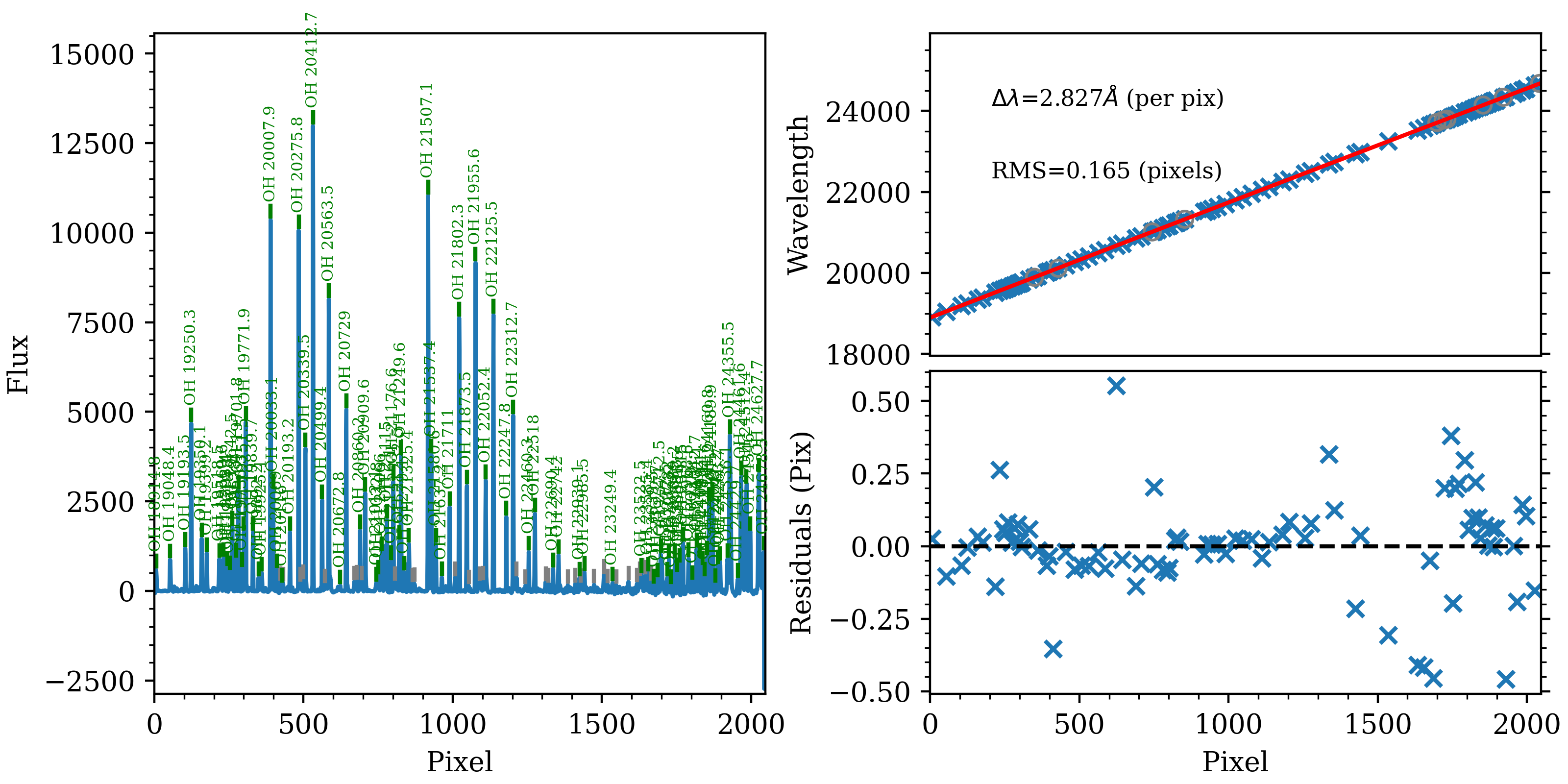
The wavelength-calibration QA plot for the reddest Keck/NIRES order
(order=3), called Arc_1dfit_A_2_DET01_S0003.png. The left panel shows
the arc spectrum extracted down the center of the order, with green text and
lines marking lines used by the wavelength calibration. Gray lines mark
detected features that were not included in the wavelength solution. The
top-right panel shows the fit (red) to the observed trend in wavelength as a
function of spectral pixel (blue crosses); gray circles are features that
were rejected by the wavelength solution. The bottom-right panel shows the
fit residuals (i.e., data - model).
In addition, the script pypeit_chk_wavecalib provides a summary of the wavelength calibration for all orders. We can run it with this simple call:
pypeit_chk_wavecalib Calibrations/WaveCalib_A_2_DET01.fits
and it prints on screen the following (you may need to expand the width of your terminal to see the full output):
 N. SpatID minWave Wave_cen maxWave dWave Nlin     IDs_Wave_range    IDs_Wave_cov(%) measured_fwhm  RMS
--- ------ ------- -------- ------- ----- ---- --------------------- --------------- ------------- -----
  0    234  8131.7   9408.9 10646.5 1.225   30  9793.676 - 10527.657            29.2           2.1 0.085
  1    416  9496.8  10961.4 12401.6 1.419   91  9793.676 - 12351.597            88.1           2.1 0.078
  2    574 11380.8  13133.2 14860.1 1.699   95 11439.783 - 14833.093            97.5           2.1 0.129
  3    720 14203.1  16389.5 18547.8 2.122  106 14227.201 - 18526.181            98.9           2.2 0.106
  4    885 18895.7  21806.9 24686.8 2.827   84 18914.824 - 24627.748            98.6           2.0 0.165
See pypeit_chk_wavecalib for a detailed description of all the columns.
Warning
A common failure mode for wavelength calibration that uses the sky lines is that the exposures are too short. When collecting NIRES observations, either (1) make sure at least some of the on-sky exposures are sufficiently long to provide good signal in the sky lines in all orders or (2) take arc lamp exposures. If you’ve already collected your data and you didn’t do either of these, you can try using archive observations or ask the Keck staff to take arc lamps for you, given that NIRES is a fixed-format spectrograph.
PypeIt currently does not have a pre-cooked arc-lamp wavelength solution for NIRES. If you want to perform wavelength calibration with arc lamp spectra, you’ll need to change the default approach; see Wavelength Calibration, and see KECK NIRES (keck_nires) for the current default wavelength calibration approach.
2D Wavelength Solution
Finally, PypeIt traces the position of each spectral line as a function of the spatial position within each order to create a 2D wavelength solution for the slit/order image. The primary QA plot for this shows the measured and modeled locations of each line.
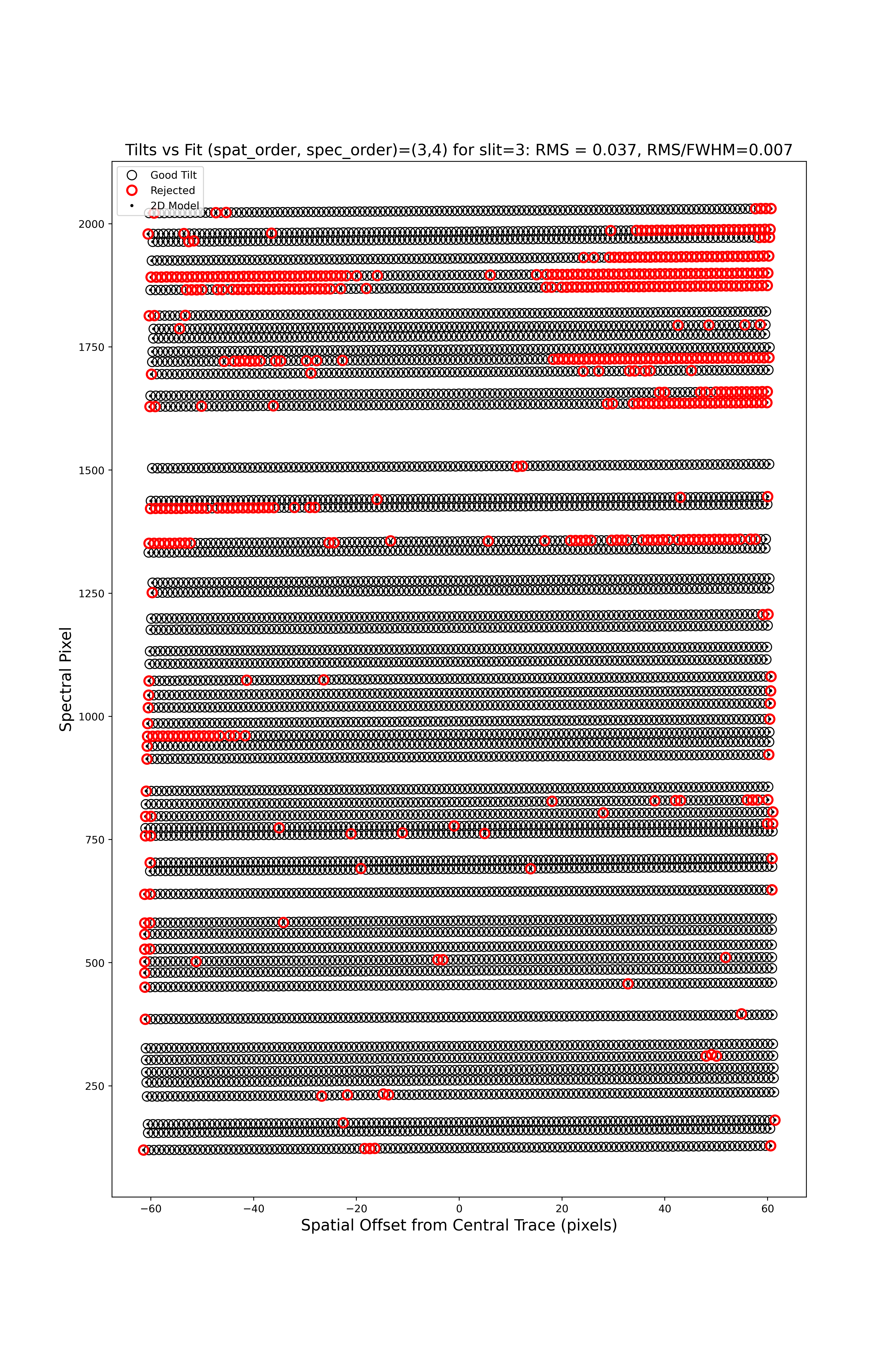
The 2D wavelength-calibration QA plot for the reddest Keck/NIRES order (order=3). Each open circle is the measured center of an arc (sky) line; black circles are included in the 2D model, whereas red circles have been rejected. Black points show the model predicted position. The text across the top of the figure gives the RMS of the 2D wavelength solution, which should be less than 0.1 pixels.
Field Flattening
PypeIt computes a number of multiplicative corrections to correct the 2D spectral response for pixel-to-pixel detector throughput variations and lower-order spatial and spectral illumination and throughput corrections. We collectively refer to these as flat-field corrections; see here and here. For NIRES observations, flats with lamps off, if available, are also subtracted.
You can inspect the flat-field corrections using the following script:
pypeit_chk_flats Calibrations/Flat_A_7_DET01.fits
Note that the calibration group number for this image is 7 (instead of 2 or
4) because the flat field images were used for all calibration groups. The
first channel in the resulting ginga window looks as follows:
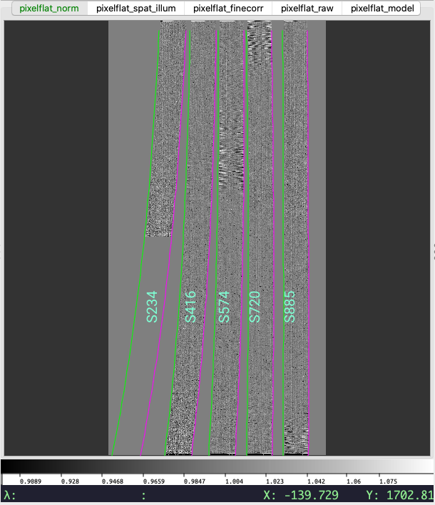
The first channel (pixelflat_norm) in the PypeIt flat-field calibration,
showing the normalized pixel flat. The edges of the slits are marked the
same as for the trace image (see above). The values in this image should all
be near unity.
Object Finding and Extraction
After the above calibrations are complete, PypeIt will iteratively identify sources, perform local and global sky subtraction, and perform 1D spectral extractions. This process is fully described here: Object Finding.
PypeIt produces QA files that allow you to assess the detection of the objects. For example, here is the QA plot for the faint object found in order 3:
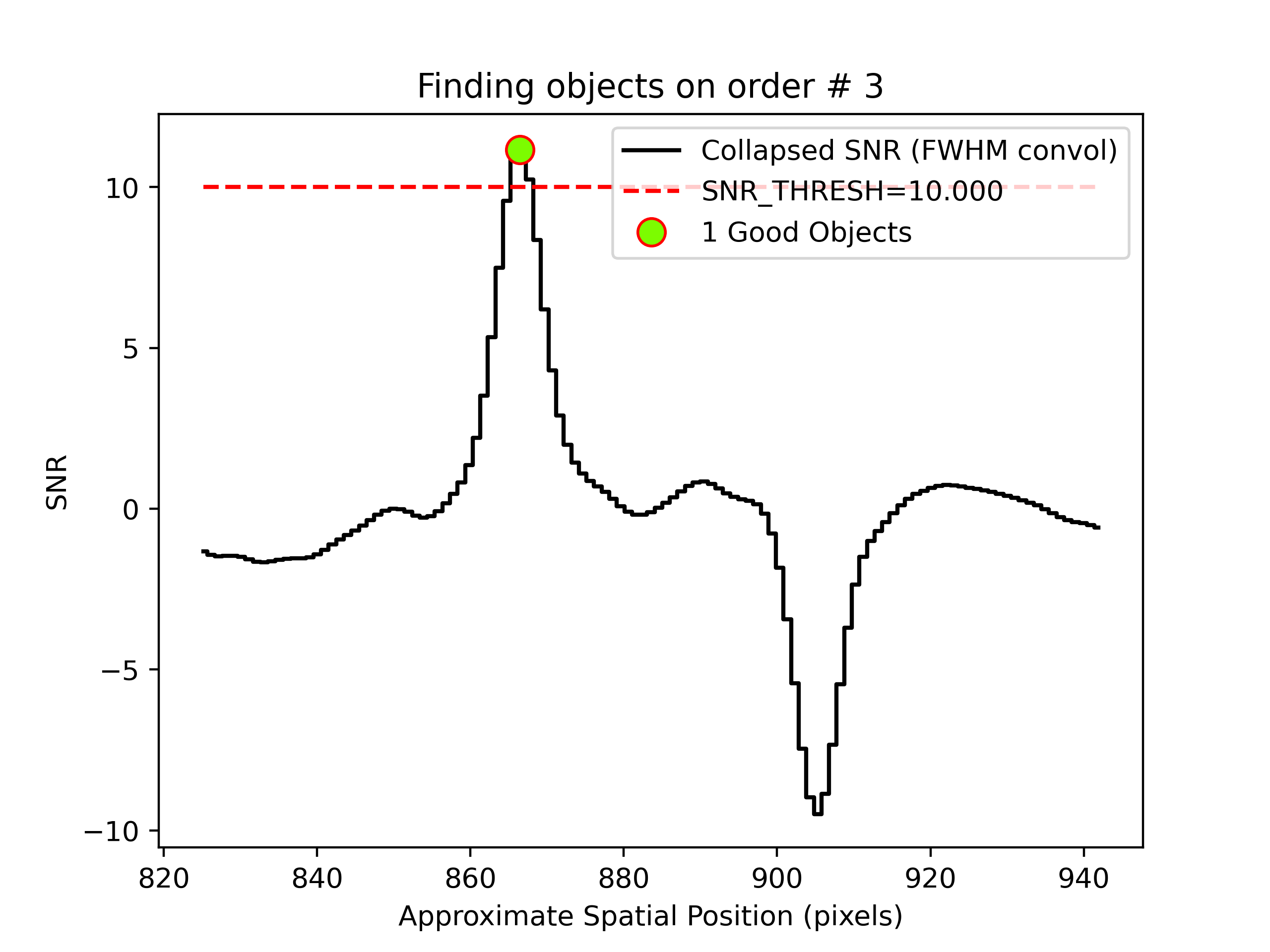
Detection of a source spectrum in order 3. The black line shows the
spectrally collapsed S/N as a function of position within the slit/order.
The dashed red line is the S/N threshold set by the FindObjPar Keywords, and
the green circle marks the spatial position of the detected object. The name
of this file is
pos_s190519_0068-J1450+3302_NIRES_20190519T095754.265_DET01_S0003_obj_prof.png.
We are using difference imaging, so PypeIt produces such plots for both the positive and negative traces. Also, given that NIRES produces multi-order echelle data, PypeIt will attempt to extract the object spectrum across all orders, even if it is only detected in a single order. Here, PypeIt uses the provided standard spectrum as a crutch to trace the relative spatial position of the faint object spectrum in all orders, even though it is only detected with S/N > 10 in the reddest order.
Core Processing Outputs
The primary science output from run_pypeit are 2D spectral images and 1D spectral extractions; see Outputs.
2D Spectral Images
Each “combination group” will produce a calibrated 2D spectral image; see
Spec2D Output for more information about these images. In this example,
each science and standard frame are assigned their own unique combination group
(comb_id in the pypeit file). For A-B differencing, an image is typically
created for each dither position, which can be combined using our 2D coadding
algorithms (see Coadd 2D Spectra).
The calibrated 2D spectral images can be visually inspected using pypeit_show_2dspec, which displays the images in a ginga window. For example, the figure below shows 3 of the 4 image channels derived from one of the standard star observations, displayed by executing:
pypeit_show_2dspec Science/spec2d_s190519_0059-GD153_NIRES_20190519T083811.995.fits --removetrace
The --removetrace option is particularly useful for faint sources; this
option only shows the object trace in the first channel (the channel showing the
calibrated science image), but does not include it in the remaining 3 channels.
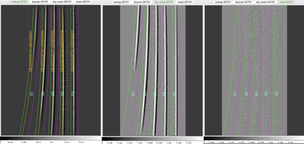
Three of the four ginga channels displayed when using
pypeit_show_2dspec for one of the standard star frames. Specifically,
this is the A-B image. Note that the object trace is only in the first
ginga channel.
The main assessments to perform are to make sure that the object is well traced
(e.g., in the sciimg channel), that there are little to no strong sky
residuals in the sky_resid channel, and that the data in the resid
channel looks like pure noise (see also pypeit_chk_noise_2dspec).
1D Spectral Extractions
Each “combination group” will also produce a fits file containing 1D spectral
extractions; see Spec1D Output for more information about these files
(including the nameing convention). The name of the file is:
spec1d_s190519_0059-GD153_NIRES_20190519T083811.995.fits. An ASCII text
file, named spec1d_s190519_0059-GD153_NIRES_20190519T083811.995.txt (i.e.,
the same name but with the extension changed from .fits to .txt), is also
produced that provides a summary of the extracted spectra. For the same
standard star frame shown above, the file looks like this:
| order |          name | spat_pixpos | spat_fracpos | box_width | opt_fwhm |   s2n | wv_rms |
|     7 | OBJ0355-DET01 |       215.0 |        0.355 |      1.50 |    0.965 |  0.00 |  0.085 |
|     6 | OBJ0355-DET01 |       398.3 |        0.355 |      1.50 |    0.903 | 61.86 |  0.078 |
|     5 | OBJ0355-DET01 |       556.4 |        0.355 |      1.50 |    0.877 | 51.53 |  0.129 |
|     4 | OBJ0355-DET01 |       702.7 |        0.355 |      1.50 |    0.878 | 51.61 |  0.106 |
|     3 | OBJ0355-DET01 |       867.7 |        0.355 |      1.50 |    0.764 | 31.38 |  0.165 |
This shows that a single spectrum was extracted for each order. Each spectrum is given its own extension in the fits file, where the extension name is based on the object name identified in the file and the order number; e.g., OBJ0355-DET01-ORDER0007.
You can plot the spectrum using pypeit_show_1dspec:
pypeit_show_1dspec Science/spec1d_s190519_0059-GD153_NIRES_20190519T083811.995.fits --exten 9
The --exten 9 argument specifies to use the fifth extension in the fits file, which selects the reddest (order=3) spectrum.
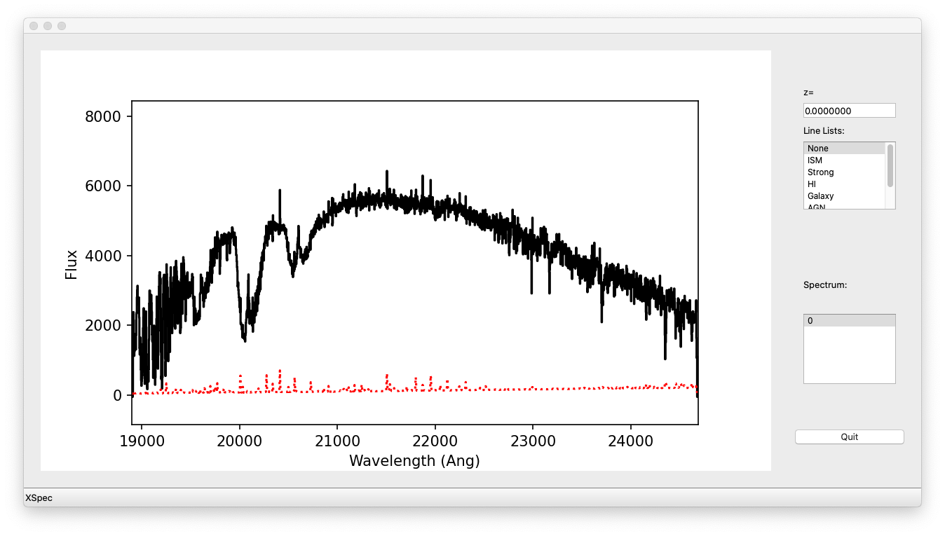
See Spec1D Output for further details.
2D Coadding
The main reduction of this Keck/NIRES dataset produces two output spectra, one
for the A-B frame and one for the B-A frame. To combine these 2D
spectra, we suggest using pypeit_coadd_2dspec. See Coadd 2D Spectra for
more information and Coadd2D HOWTO for usage examples.