Keck-LRIS HOWTO
Overview
This doc goes through a full run of PypeIt on one of our Keck LRIS
multi-object datasets, specifically the keck_lris_red_mark4/multi_600_10000_slitmask
dataset. These are Keck LRIS RED multi-slit observations taken with the new
Mark IV detector and the 600/10000 grating. See here
to find the example dataset.
Note
This doc shows the reduction steps for a multi-slit dataset. For long-slit datasets, the reduction steps are the same, but the setup is considerably simpler. In the text below, we will point out the differences.
If you’re having trouble reducing your data, we encourage you to try going through this tutorial using this example dataset first. Please join our PypeIt Users Slack using this invitation link to ask for help, and/or Submit an issue to Github if you find a bug!
The following was performed on a Macbook Pro with 16 GB RAM and took approximately 30 minutes.
Setup
Organize data
Identify the folder where the raw data are stored and make sure you have
all the calibration files you need, in addition to the science ones.
In this example, the raw data are stored in the folder
/PypeIt-development-suite/RAW_DATA/keck_lris_red_mark4/multi_600_10000_slitmask.
The files within this folder are:
$ ls -1
r230417_01033.fits
r230417_01064.fits
r230417_01072_with_maskinfo.fits
This folder can include data from different datasets (e.g., more than one slitmask or observations in various gratings). The script pypeit_setup (see next step) will help to parse the desired dataset.
Note
The following is only for multi-slit datasets. For long-slit observations, the user can skip this step.
Pypeit is able to incorporate slitmask information in the reduction routine,
(similarly to how it is done for Keck/DEIMOS observations).
However, unlike DEIMOS, LRIS slitmask information is not included in the raw data,
and the user needs to add it to the raw data before running PypeIt. The software
TILSOTUA can help with that, but the
user needs first to obtain the mask design files. The files needed are two
output files produced by autoslit
when creating the slitmask for the observations, and The ASCII object list file fed as input to
autoslit. Those files are processed by
TILSOTUA and converted into binary tables, containing the slitmask design information,
the object catalog and the mapping between the two. The user, subsequently, needs to
append the binary tables to the raw flat field image file. See Slit-masks
for more details. In this example, the raw file r230417_01072_with_maskinfo.fits
already includes the slitmask information.
If the slitmask information is not found in the raw data file, Pypeit will still be able to reduce the data but will not be able to use the slitmask information.
Run pypeit_setup
The first script to run with PypeIt is pypeit_setup, which examines the raw files and generates a sorted list and (when instructed) one PypeIt Reduction File per instrument configuration.
See complete instructions provided in Setup.
Important
Know the spectrograph you need to use! LRIS went through different upgrades
(FITS file format and detectors, see Keck LRIS) and PypeIt uses different spectrograph
names to differentiate between them. In this example, we are using observations taken
with the new Mark IV detector in the red arm, so we use the spectrograph name
keck_lris_red_mark4. PypeIt will throw an error if you use the wrong LRIS spectrograph name.
For this example, we move to the folder where we want to perform the reduction and save the associated outputs and we run:
cd folder_for_reducing
pypeit_setup -s keck_lris_red_mark4 -r /PypeIt-development-suite/RAW_DATA/keck_lris_red_mark4/multi_600_10000_slitmask
This creates, in a folder called setup_files/, a .sorted file that shows the raw files organized
by datasets. We inspect the .sorted file and identify the dataset that we want to reduced
(in this case it is indicated with the letter A ) and re-run pypeit_setup as:
pypeit_setup -s keck_lris_red_mark4 -r /PypeIt-development-suite/RAW_DATA/keck_lris_red_mark4/multi_600_10000_slitmask -c A
This creates a PypeIt Reduction File called keck_lris_red_mark4_A.pypeit inside a folder called
keck_lris_red_mark4_A/, and it looks like this:
# Auto-generated PypeIt input file using PypeIt version: 1.14.1.dev432+gf9a4a24da
# UTC 2023-12-08T19:35:05.109

# User-defined execution parameters
[rdx]
    spectrograph = keck_lris_red_mark4

# Setup
setup read
Setup A:
  amp: '4'
  binning: 2,2
  cenwave: 8081.849304
  decker: frb22022
  dichroic: '680'
  dispangle: 29.418736
  dispname: 600/10000
setup end

# Data block
data read
 path /PypeIt-development-suite/RAW_DATA/keck_lris_red_mark4/multi_600_10000_slitmask
                        filename |                 frametype |                 ra |                 dec |     target |  dispname |   decker | binning |          mjd | airmass |       exptime | dichroic | amp | dispangle |     cenwave |  hatch |                  lampstat01 |    dateobs | frameno | calib
              r230417_01064.fits |                  arc,tilt | 229.99999999999997 |                45.0 | DOME FLATS | 600/10000 | frb22022 |     2,2 | 60051.725892 |    1.41 |   1.000125952 |      680 |   4 | 29.417606 | 8081.269988 | closed | HgI NeI ArI CdI ZnI KrI XeI | 2023-04-17 |    1064 |     0
r230417_01072_with_maskinfo.fits | pixelflat,illumflat,trace | 229.99999999999997 |                45.0 | DOME FLATS | 600/10000 | frb22022 |     2,2 | 60051.729634 |    1.41 |  10.000135168 |      680 |   4 | 29.417606 | 8081.269988 |   open |                          on | 2023-04-17 |    1072 |     0
              r230417_01033.fits |                   science |          203.90275 | -28.032416666666666 |   frb22022 | 600/10000 | frb22022 |     2,2 | 60051.349105 |    1.71 | 500.000625152 |      680 |   4 | 29.418736 | 8081.849304 |   open |                         off | 2023-04-17 |    1033 |     0
data end
Inspecting this file, we want to make sure that all the frame types were accurately assigned in the
Data Block. If not, these can be fixed by editing the PypeIt Reduction File directly; see instructions
here. We can also remove any bad (or undesired) calibration
or science frames from the list, by either deleting them altogether or commenting them out with a #.
In this example, all the frametypes were accurately assigned. We only make edits to the Parameter Block. The edited version looks like this (pulled directly from the PypeIt Development Suite):
# Auto-generated PypeIt input file using PypeIt version: 1.12.3.dev7+ga9075153d
# UTC 2023-05-08T19:54:58.446

# User-defined execution parameters
[rdx]
    spectrograph = keck_lris_red_mark4
[baseprocess]
    use_biasimage = False
[calibrations]
 [[slitedges]]
   use_maskdesign = True
[reduce]
 [[slitmask]]
    use_alignbox = False
    assign_obj = True
    extract_missing_objs = True
  [[findobj]]
    snr_thresh = 3.0
  [[extraction]]
    use_2dmodel_mask = False

# Setup
setup read
Setup A:
  amp: '4'
  binning: 2,2
  cenwave: 8081.849304
  decker: frb22022
  dichroic: '680'
  dispangle: 29.418736
  dispname: 600/10000
setup end

# Data block
data read
# path PypeIt-development-suite/RAW_DATA/keck_lris_red_mark4/multi_600_10000_slitmask
 path multi_600_10000_slitmask
                        filename |                 frametype |                 ra |                 dec |     target |  dispname |   decker | binning |          mjd | airmass |       exptime | dichroic | amp | dispangle |     cenwave |  hatch |                  lampstat01 |    dateobs | frameno | calib
              r230417_01064.fits |                  arc,tilt | 229.99999999999997 |                45.0 | DOME FLATS | 600/10000 | frb22022 |     2,2 | 60051.725892 |    1.41 |   1.000125952 |      680 |   4 | 29.417606 | 8081.269988 | closed | HgI NeI ArI CdI ZnI KrI XeI | 2023-04-17 |    1064 |     0
r230417_01072_with_maskinfo.fits | pixelflat,illumflat,trace | 229.99999999999997 |                45.0 | DOME FLATS | 600/10000 | frb22022 |     2,2 | 60051.729634 |    1.41 |  10.000135168 |      680 |   4 | 29.417606 | 8081.269988 |   open |                          on | 2023-04-17 |    1072 |     0
              r230417_01033.fits |                   science |          203.90275 | -28.032416666666666 |   frb22022 | 600/10000 | frb22022 |     2,2 | 60051.349105 |    1.71 | 500.000625152 |      680 |   4 | 29.418736 | 8081.849304 |   open |                         off | 2023-04-17 |    1033 |     0
data end
The parameters use_maskdesign, use_alignbox, assign_obj, and extract_missing_objs
are all parameters that are specific to the slitmask design ingestion (see Slitmask ID assignment and missing slits,
RA, Dec and object name assignment to 1D extracted spectra, and Object position on the slit from slitmask design). These are not used for long-slit
observations, therefore the user can ignore them.
The other parameters are set to improve the object finding and extraction, and to instruct PypeIt not to use bias frames for the reduction (given that no bias frames are provided). See User-level Parameters for more details.
Note
PypeIt has a long list of parameters that can be set by the user to customize the reduction. This
makes PypeIt very flexible and able to reduce a wide range of data from many instruments. Most
parameters are set by default for the specific instrument, see KECK LRISr (keck_lris_red_mark4).
Moreover, there are some parameters that are set by default for a specific configuration within
the same instrument. For example, in many cases, PypeIt uses by default different wavelength templates
for different gratings (see Wavelength Solution). The default parameters are not shown in the
PypeIt Reduction File, therefore it may be sometime difficult to know which parameters to set
and which ones to leave as default.
To help with this, the user can inspect the .par file, which is generated at the very beginning
of the main run (see below). This file contains every single available parameter with the assigned
value, giving the user an idea of what are the values of the default parameters.
Main Run
Once the PypeIt Reduction File is ready, the main call is simply:
cd keck_lris_red_mark4_A
run_pypeit keck_lris_red_mark4_A.pypeit -o
The -o flag indicates that any existing output files should be overwritten. As
there are none, it is superfluous but we recommend (almost) always using it.
The code will run uninterrupted until the basic data-reduction procedures (wavelength calibration, field flattening, object finding, sky subtraction, and spectral extraction) are complete; see PypeIt’s Core Data Reduction Executable and Workflow.
As the code processes the data, it will produce a number of files and QA plots that can be inspected. A number of Inspection Scripts are available to help with this process. We present some of these below.
Calibrations
Slit Edges
The code first uses the trace frames to find the slit edges on the detector.
When available, the slitmask design information is used to help find the slit edges
(not for long-slit observations).
To check that PypeIt correctly identified every slits, we can run the pypeit_chk_edges script, with this explicit call:
pypeit_chk_edges Calibrations/Edges_A_0_DET01.fits.gz
which opens the ginga image viewer. Here is a zoom-in screenshot from the first tab in the ginga window:
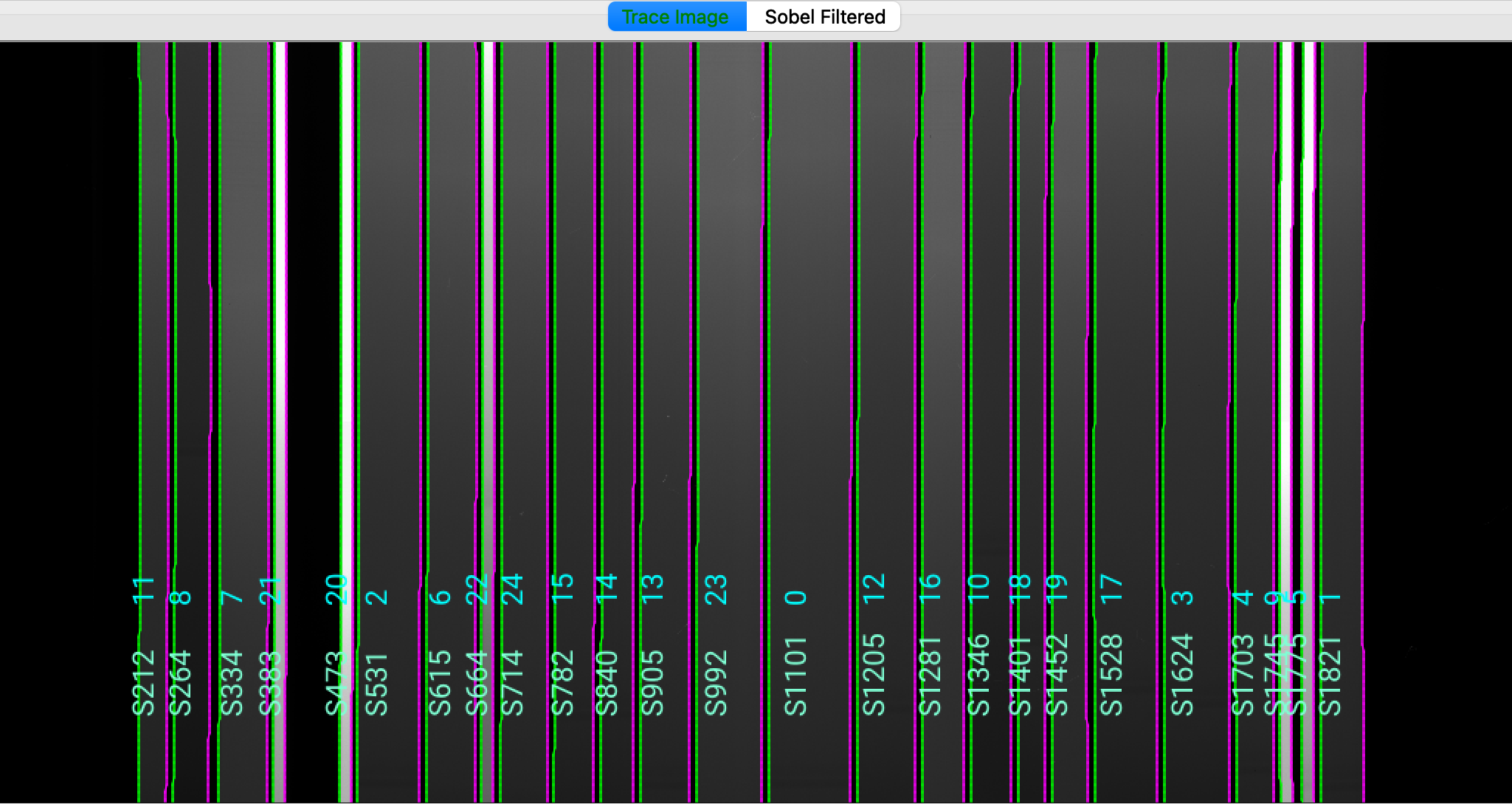
The data shown is the Trace Image, i.e., the flat image.
The green/magenta lines indicate the left/right slit edges. The aquamarine labels starting with an
S are the internal slit identifiers of PypeIt, while the cyan numbers are the slit ID values
from the slitmask design, which within the Pypeit framework are called maskdef_id. The
maskdef_id values are never shown for long-slit observations.
See Edges for further details.
We can also inspect the Slits file, which contains the main information on the traced slit edges,
organized into left-right slit pairs. This is a FITS file containing one or two astropy.io.fits.BinTableHDU
extensions. The second extension, called MASKDEF_DESIGNTAB, which is available only for multi-slit observations
and if the slitmask design information is provided, contains all the relevant slitmask design information.
In this example, the first few rows of MASKDEF_DESIGNTAB looks like this:
from astropy.io import fits
from astropy.table import Table

hdu=fits.open('Calibrations/Slits_A_0_DET01.fits.gz')
Table(hdu['MASKDEF_DESIGNTAB'].data)

TRACEID TRACESROW     TRACELPIX          TRACERPIX      SPAT_ID MASKDEF_ID SLITLMASKDEF SLITRMASKDEF       SLITRA             SLITDEC            SLITLEN            SLITWID             SLITPA       ALIGN OBJID       OBJRA               OBJDEC       OBJNAME   OBJMAG OBJMAG_BAND    OBJ_TOPDIST        OBJ_BOTDIST
 int64    int64        float64            float64        int64    int64      float64      float64         float64             float64            float64            float64            float64       int16 int64      float64             float64        str32   float64    str32         float64            float64
------- --------- ------------------ ------------------ ------- ---------- ------------ ------------ ------------------ ------------------- ------------------ ------------------ ------------------ ----- ----- ------------------ ------------------- -------- ------- ----------- ------------------ ------------------
      0      1032 193.60062170028687 231.29763960838318     212         11        211.0        247.0 203.89075232578443 -28.092169267295024  9.822391510009766 0.9919275641441345 15.412363052368164     0    11 203.89072727254896  -28.09230361665466   gal172  22.353           r  4.424071886416087  5.398871433622549
      1      1032 241.12293437753794 288.52713346481323     265          8        257.0        306.0  203.8415716281879  -28.07607209753345 13.274372100830078 0.9922505021095276 15.440143585205078     0     8 203.84147689509808 -28.076401475507694   gal227  22.567           r  5.414064692172961  7.860407169533709
      2      1032   302.332216322422 367.47612684965134     335          7        318.0        382.0  203.9166660875971 -28.089147654373047 17.321680068969727 0.9887152314186096 15.405740737915039     0     7 203.91661609856362 -28.089363864800017   gal158  21.796           r  7.868456854365888   9.45355797935212
      3      1032 375.55078342556953  391.8777657151222     384         21        392.0        407.0  203.8961977293406 -28.080303275622498  3.998490333557129 3.9599761962890625 15.393735885620117     1    21 203.89621037750157 -28.080305533949872    star6  15.653           r 2.0029598959835964  1.996361115945478
      4      1032  465.5582481622696 481.88689267635345     474         20        480.0        495.0 203.92635312081273 -28.080791243205006 3.9996068477630615 3.9622230529785156 15.388344764709473     1    20 203.92636894459946 -28.080795440193242   star10  15.728           r  1.999165077712833  2.001801640220989
See Slits for a description of all the columns of this table.
Arc
You can view the Arc image used for the wavelength calibration of the science frame with ginga:
ginga Calibrations/Arc_A_0_DET01.fits
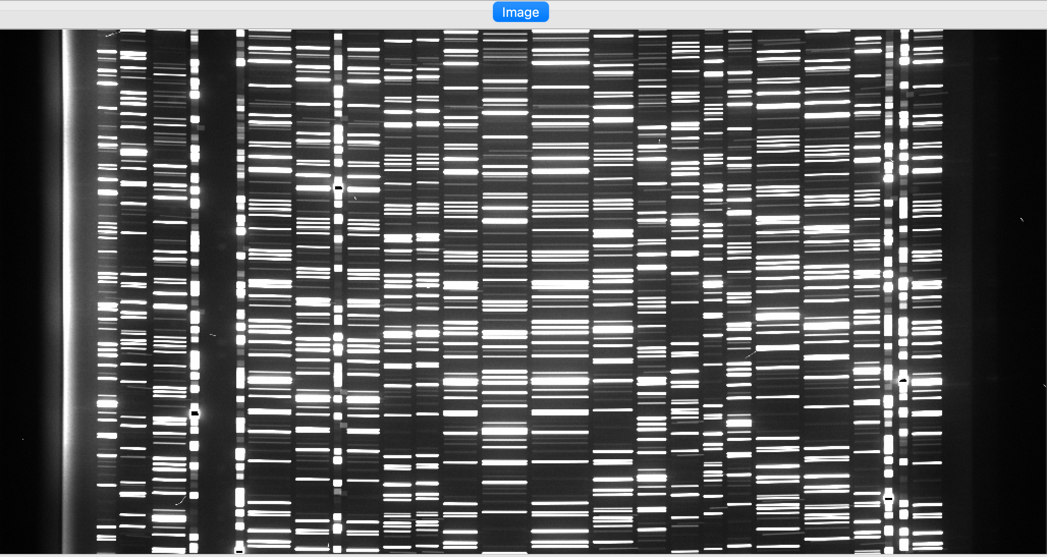
As typical of most arc images, we can see a series of arc lines, here oriented approximately horizontally. It is important to inspect the arc image to make sure it looks good, ensuring to get a good wavelength calibration.
See Arc for further details.
Wavelengths
It is, also, very important to inspect the PypeIt QA for the wavelength calibration.
These are PNG files in the QA/PNG/ folder.
1D
Here is an example of the 1D fits for one of the slit on the detector,
written to the QA/PNGs/Arc_1dfit_A_0_DET01_S0212.png file:
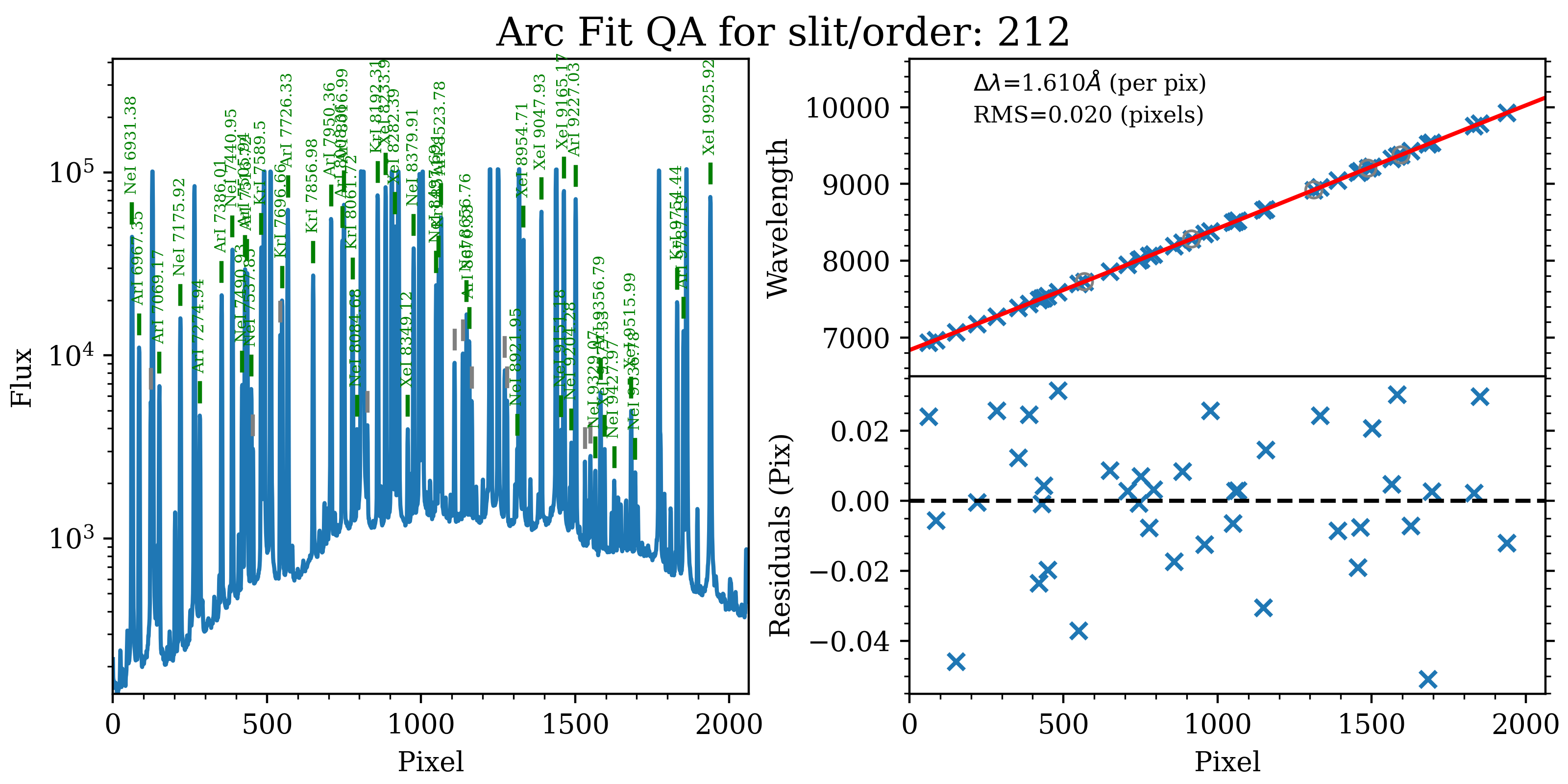
The left panel shows the arc spectrum extracted down the center of the slit, with the lines used by the wavelength calibration marked in green. Gray lines mark detected features that were not included in the wavelength solution. The top-right panel shows the fit (red) to the observed trend in wavelength as a function of spectral pixel (blue crosses); gray circles are features that were rejected by the wavelength solution. The bottom-right panel shows the fit residuals (i.e., data - model).
What you hope to see in this QA is:
On the left, many of the arc lines marked with green IDs
In the upper right, an RMS < 0.1 pixels
In the lower right, a random scatter about 0 residuals
In addition, the script pypeit_chk_wavecalib provides a summary of the wavelength calibration for all the spectra. We can run it with this simple call:
pypeit_chk_wavecalib Calibrations/WaveCalib_A_0_DET01.fits
and it prints on screen the following (here truncated) table:
 N. SpatID minWave Wave_cen maxWave dWave Nlin     IDs_Wave_range    IDs_Wave_cov(%) measured_fwhm  RMS
--- ------ ------- -------- ------- ----- ---- --------------------- --------------- ------------- -----
  0    212  6835.4   8469.9 10121.3 1.610   43  6931.379 -  9925.919            91.1           2.7 0.027
  1    265  6038.3   7674.1  9327.6 1.612   45  6336.179 -  9227.030            87.9           2.7 0.025
  2    335  7169.5   8831.4 10485.5 1.611   39  7427.339 - 10472.923            91.8           2.7 0.348
  3    384     0.0      0.0     0.0 0.000    0     0.000 -     0.000             0.0           0.0 0.000
  4    474     0.0      0.0     0.0 0.000    0     0.000 -     0.000             0.0           0.0 0.000
See pypeit_chk_wavecalib for a detailed description of all the columns.
Note that the slits with SpatID 384 and 474 have all the values set to 0.0. This is because
these slits are actually alignment boxes and they are not reduced by the pipeline.
Tilts
Wavelength tilts are measured performing a 2D fit to the traced arc lines.
There are several QA files written for the 2D fits. One example is
QA/PNGs/Arc_tilts_2d_A_0_DET01_S0212.png:
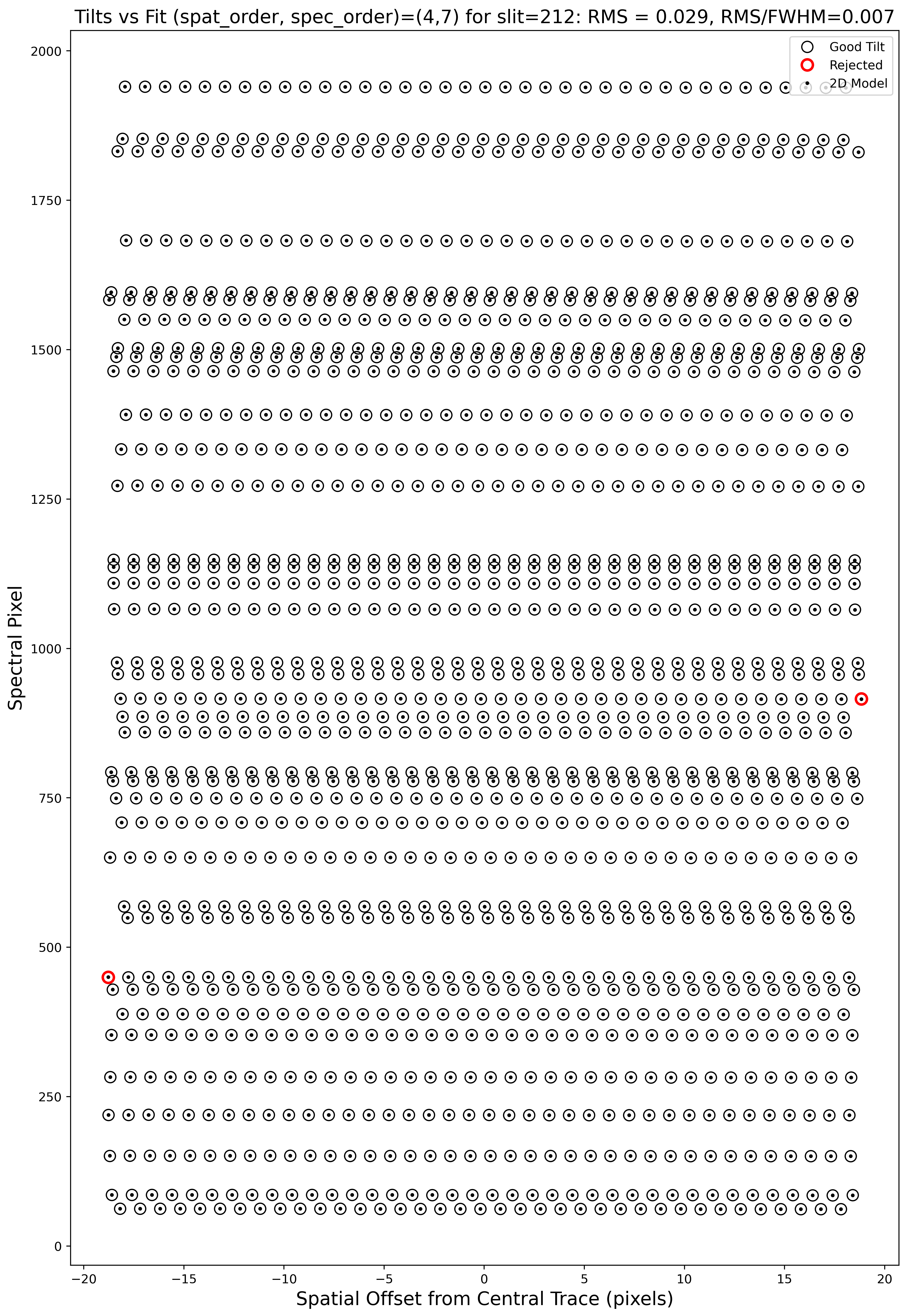
Each horizontal line of black open circles identifies a traced arc line. Red circles shows the points that were rejected in the 2D fitting, and the black points show the model predicted position. The text across the top of the figure gives the RMS of the 2D wavelength solution, which should be less than 0.1 pixels.
The 2D fit for the wavelength tilts can also be inspected using the script pypeit_chk_tilts, which shows a Tiltimg image in a ginga or matplotlib window with the traced and 2D fitted tilts over-plotted. Here is an example:
pypeit_chk_tilts Calibrations/Tilts_A_0_DET01.fits
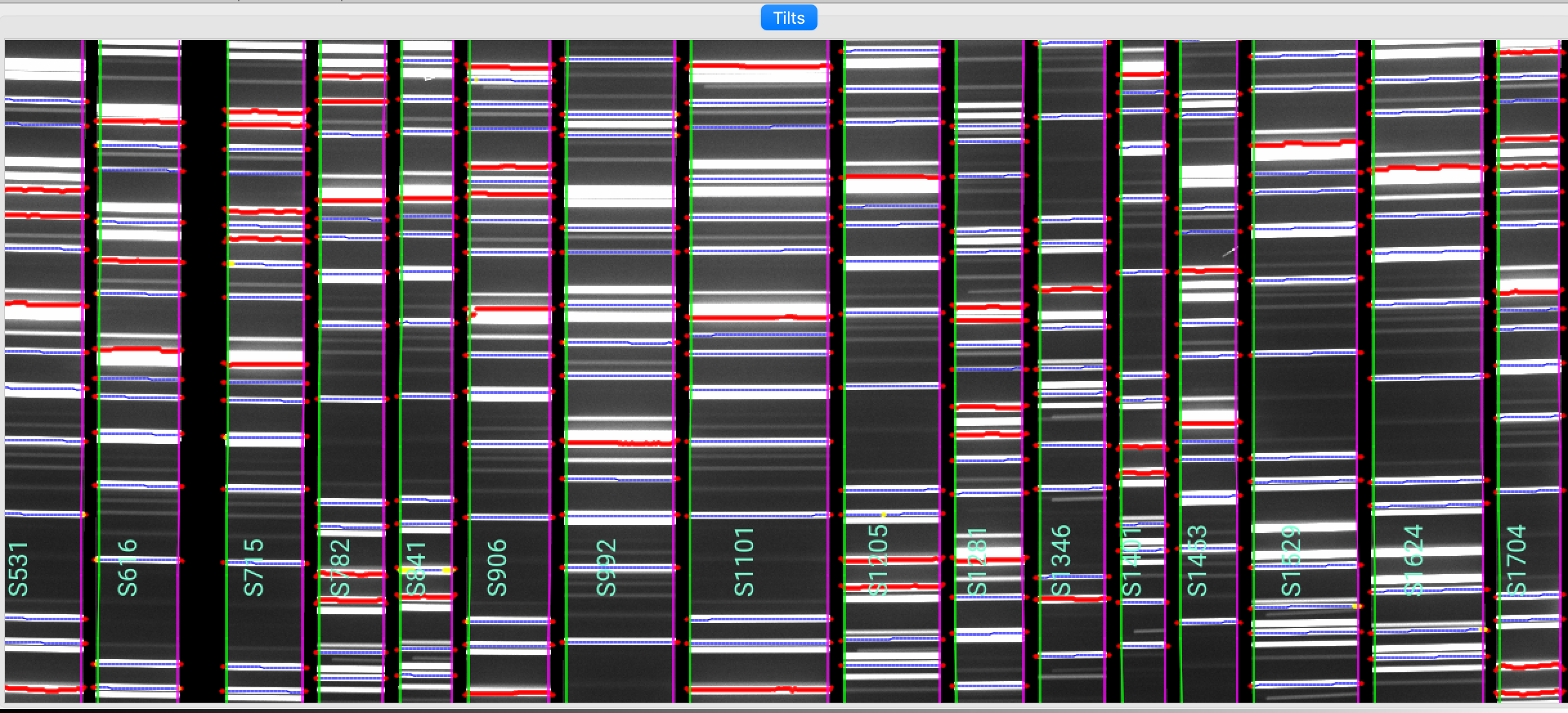
This shows a zoom-in of a Tiltimg image in a ginga window with overlaid the 2D fitted tilts (blue), the masked pixels (red), and the pixels rejected in the 2D fitting (yellow). The lines that are not overlaid with any colored tilts are the ones that were not detected for the purpose of the performing the 2D fitting.
See Tilts for further details.
Flatfield
PypeIt computes a number of multiplicative corrections to correct the 2D spectral response
for pixel-to-pixel detector throughput variations and lower-order spatial and spectral illumination
and throughput corrections. We collectively refer to these as flat-field corrections; see
here and here.
To inspect the Flat images we can use the script pypeit_chk_flats, with this explicit call:
pypeit_chk_flats Calibrations/Flat_A_0_DET01.fits
Here is a zoom-in screenshot from the first tab in the ginga window (pixflat_norm):
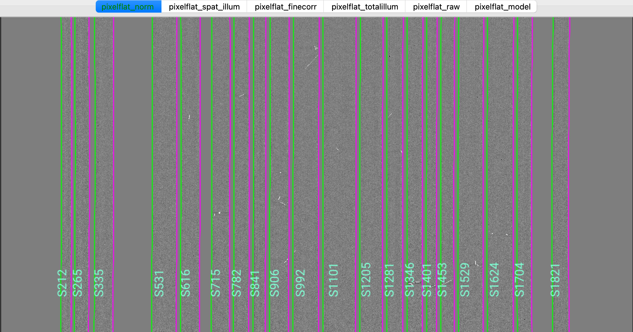
This shows the normalized flat field image. The green/magenta lines are the slit edges, which are tweaked using the illumination flat field.
See Flat and Flat Fielding for further details.
Object finding
After the above calibrations are complete, PypeIt will iteratively identify sources, perform global and local sky subtraction, and perform 1D spectral extractions. This process is fully described here: Object Finding.
PypeIt produces QA files that allow you to assess the detection of the objects.
One example is QA\PNGs\r230417_01033-frb22022_LRISr_20230417T082242.672_DET01_S0212_obj_prof.png:
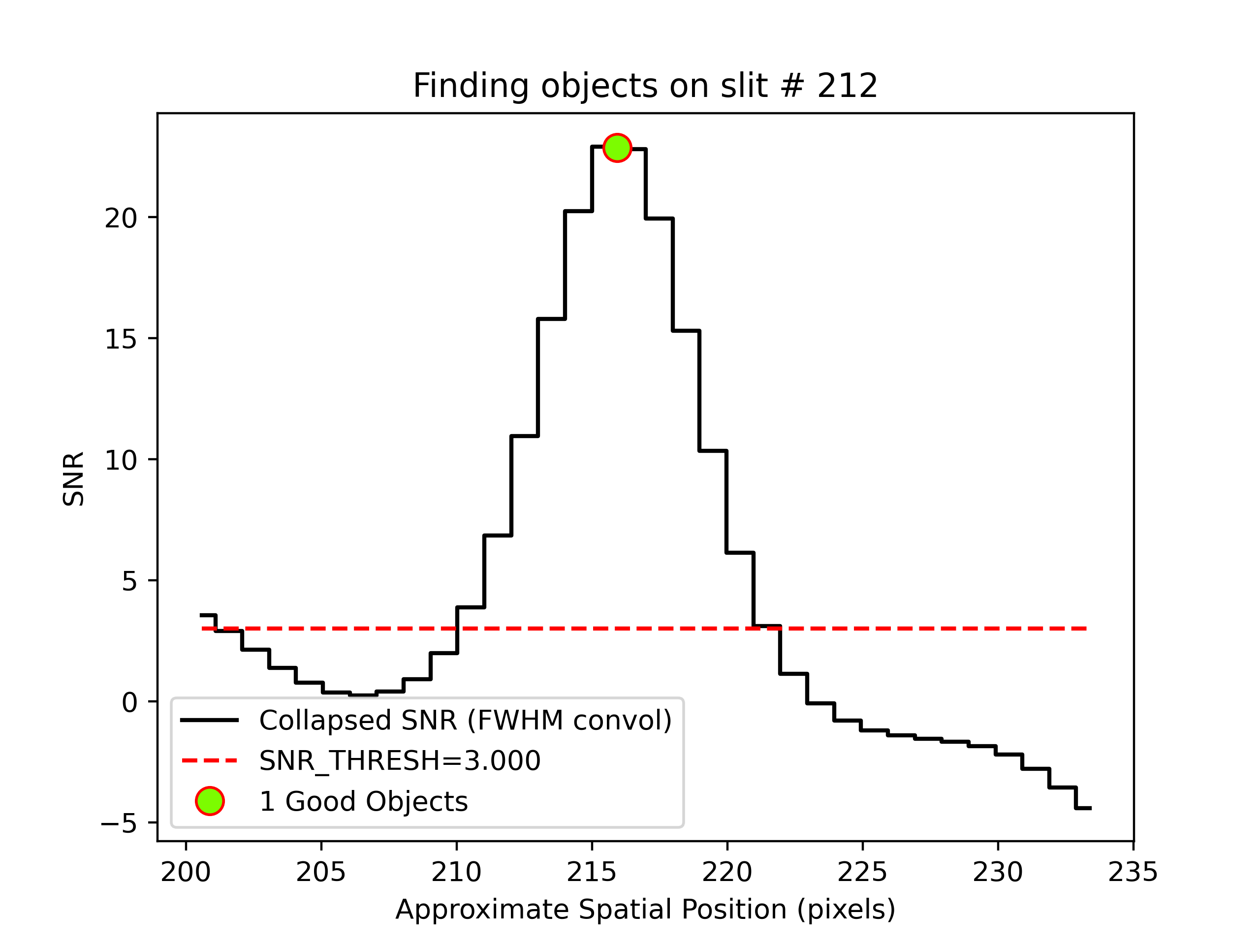
This shows the spatial profile of the object’s S/N collapsed along the spectral direction.
The dashed red line is the S/N threshold set by the FindObjPar Keywords, and the green circle
marks the spatial position of the detected object. This plot is useful to assess if the object
was correctly detected and if the S/N threshold (snr_thresh) set is appropriate for the
observation. See Object Finding for further details.
Flexure
PypeIt also measures a spectral flexure correction, by performing a cross-correlation
between the sky spectrum extracted in each slit and an archived sky spectrum.
The relative shift between the two spectra is then used to correct the wavelength solution
for each slit (see Spectral Flexure).
Two flexure corrections are computed, one (called global) using the sky lines
extracted at the center of the slit, and one (called local) using the sky lines
extracted at the location of the science object.
There are two QA files (two for the global and two for the local correction)
that can be used to assess the flexure correction. Here is an example of two QA files
for the global correction, called
QA/PNGs/r230417_01033-frb22022_LRISr_20230417T082242.672_global_DET01_S0212_spec_flex_corr.png and
QA/PNGs/r230417_01033-frb22022_LRISr_20230417T082242.672_global_DET01_S0212_spec_flex_sky.png:
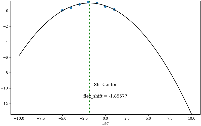
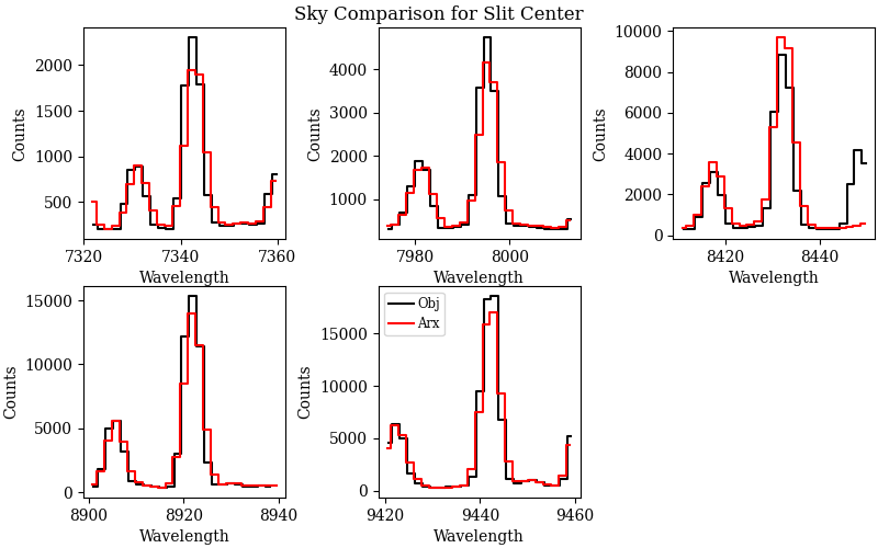
The first plot shows the polynomial fit (black line) between the top seven highest cross-correlation values (y-axis) and the corresponding shift in pixels (x-axis). The value of the shift with the highest cross-correlation is the flexure correction applied to the wavelength solution (also printed in the plot). The user should inspect this plot to make sure that the fit is good and that the value of the flexure shift is comparable to what expected for the observations. The second plot shows sky spectrum cutouts around some of the sky lines used for the flexure correction. The black line is the sky spectrum extracted at the center of the slit shifted by the computed flexure correction, while the red line is the archived sky spectrum. This is another way to assess that the computed flexure correction is good. The user should hope to see a good match between the two spectra.
Outputs
The primary science output from run_pypeit are 2D spectral images and 1D
spectral extractions, located in the Science/ folder.; see Outputs.
Spec2D
Slit inspection
It is frequently useful to view a summary of the slits successfully reduced by PypeIt, by running the script pypeit_parse_slits. In this example, we can inspect the reduced 2D spectrum with this explicit call:
pypeit_parse_slits Science/spec2d_r230417_01033-frb22022_LRISr_20230417T082242.672.fits
which print the following (here truncated) table in the terminal:
============================== DET01 ==============================
SpatID   MaskID   MaskOFF (pix)  Flags
0212     0011     0.42           None
0265     0008     0.42           None
0335     0007     0.42           None
0384     0021     0.42           BOXSLIT
0474     0020     0.42           BOXSLIT
The four columns printed to screen are SpatID (the internal PypeIt ID), MaskID,
(the slit ID from the slitmask design), MaskOFF (the dither offset) and Flags for each slit.
Slits with Flags set to BOXSLIT are alignment boxes and are not reduced by PypeIt. If the
calibration failed for some slits, the Flags column will show the reason for the failure.
Those slits with None in the Flags column have been successfully reduced.
Note that the MaskID and MaskOFF columns are not printed for long-slit observations.
Visual inspection
The 2D spectrum can be visually inspected using the script pypeit_show_2dspec. In this example, we can visualize the 2D spectrum with this explicit call:
pypeit_show_2dspec Science/spec2d_r230417_01033-frb22022_LRISr_20230417T082242.672.fits --removetrace
The --removetrace only shows the object trace in the first channel (the channel showing the
calibrated science image), but does not include it in the remaining channels. It is helpful to
to use the --removetrace option to better visualize the object traces (especially for faint
objects).
We show here a zoom-in screenshot from three (sciimg-DET01, sky_resid-DET01, resid-DET01) of the
four tabs in the ginga window:
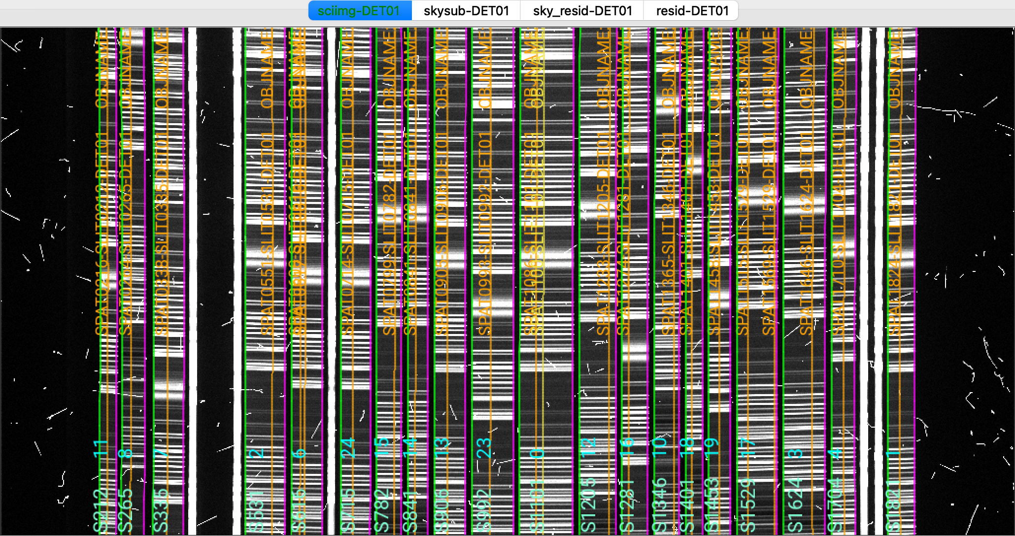
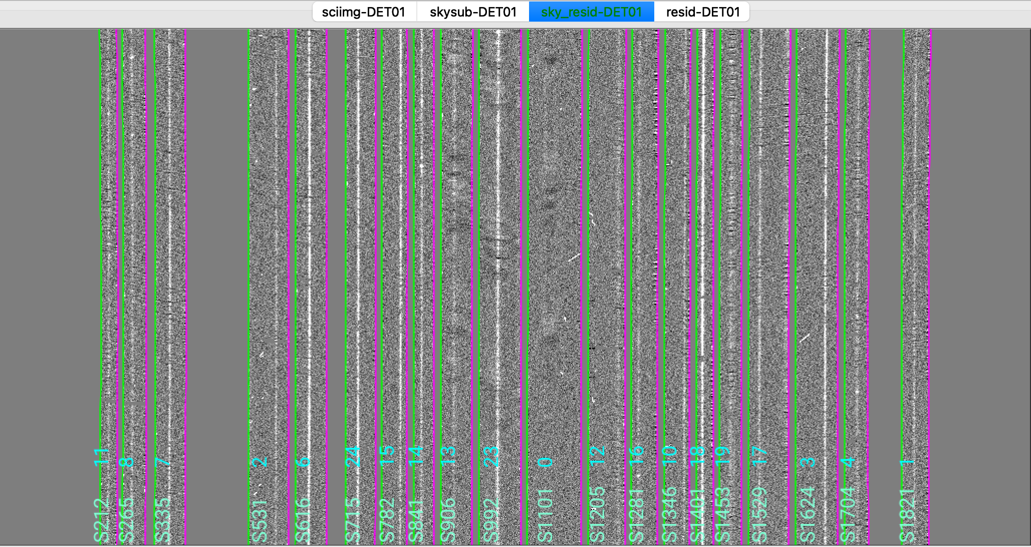
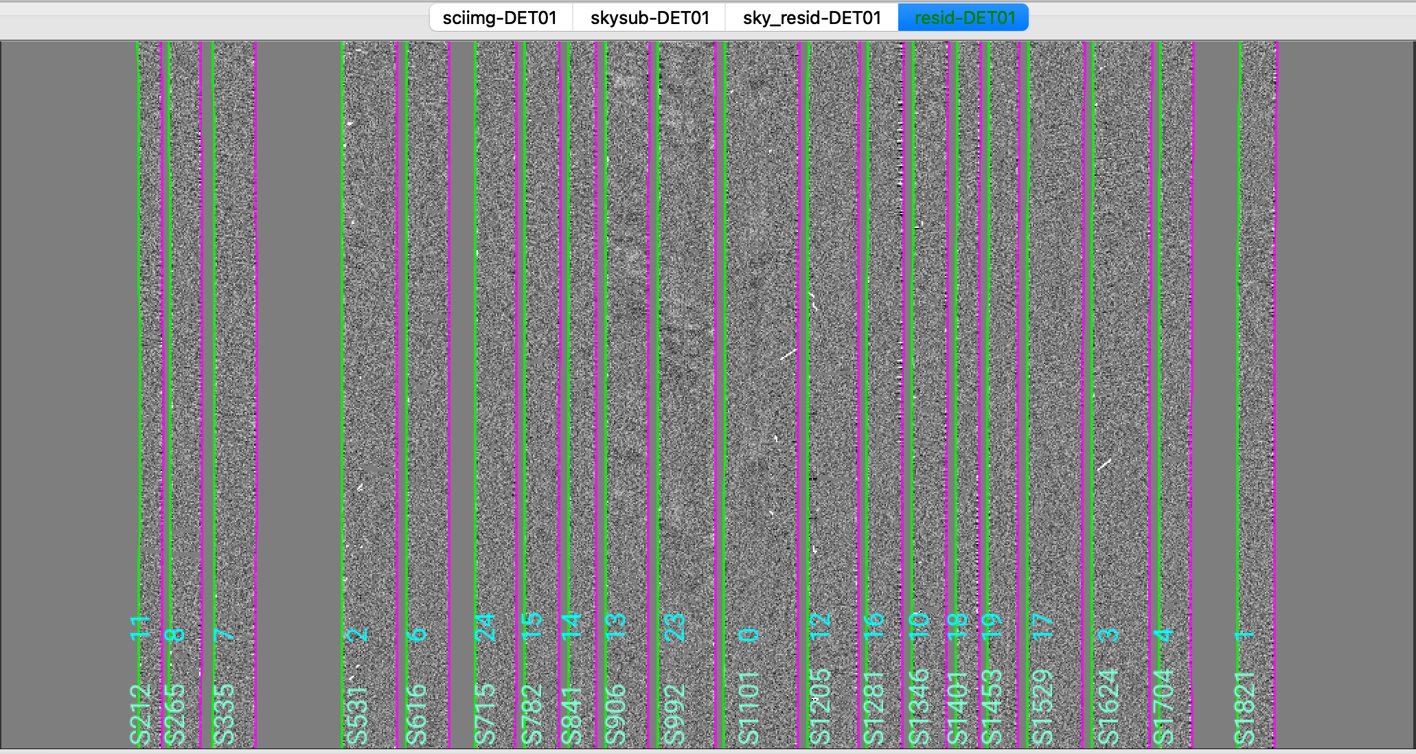
This shows on the top the calibrated science image, in the middle the sky residual image (sky-subtracted
calibrated image divided by the uncertainties), and on the right the residual image.
The green/magenta lines are the slit edges. The orange lines (shown only in the first channel)
are the object traces and the orange text is the PypeIt assigned name (starting with SPAT).
Only for multi-slit observations, and if the slitmask design information is provided,
The orange text also includes the object name from the slitmask design information (starting with OBJNAME).
Yellow lines, if present, indicate sources that, although not detected, have been extracted
at the expected location using the slitmask design information (still only for multi-slit observations).
See Spec2D Output for further details.
The main assessments to perform are to make sure that the object is well traced,
that there are little to no strong sky residuals in the sky_resid channel,
and that the data in the resid channel looks like pure noise (see also pypeit_chk_noise_2dspec).
Spec1D
You can see a summary of all the extracted sources in the spec1d*.txt files saved
in the Science/ folder. For this example, here are the first few lines of the file
Science/spec1d_r230417_01033-frb22022_LRISr_20230417T082242.672.txt:
| slit |                    name | maskdef_id |  objname |     objra |    objdec | spat_pixpos | spat_fracpos | box_width | opt_fwhm |   s2n | maskdef_extract | wv_rms |
|  212 | SPAT0216-SLIT0212-DET01 |         11 |   gal172 | 203.89073 | -28.09230 |       216.3 |        0.454 |      3.00 |    1.184 |  2.21 |           False |  0.027 |
|  265 | SPAT0264-SLIT0265-DET01 |          8 |   gal227 | 203.84148 | -28.07640 |       263.5 |        0.384 |      3.00 |    1.240 |  2.19 |           False |  0.025 |
|  335 | SPAT0338-SLIT0335-DET01 |          7 |   gal158 | 203.91662 | -28.08936 |       338.1 |        0.458 |      3.00 |    0.829 |  4.22 |           False |  0.348 |
It shows a table with the PypeIt names of the extracted spectra in each slit and all the associated information about the extraction and the object. See Extraction Information for a detailed description of this file. Note that the maskdef_id, objname, objra, objdec and maskdef_extract columns are not printed for long-slit observations.
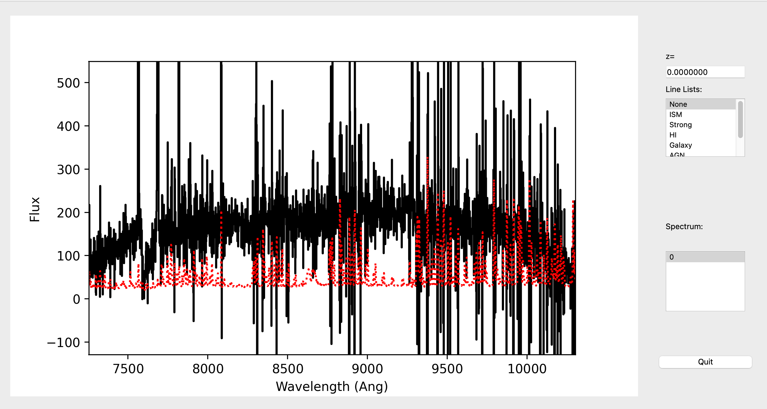
To inspect the 1D spectrum, we can use the script pypeit_show_1dspec, with a call like this:
pypeit_show_1dspec Science/spec1d_r230417_01033-frb22022_LRISr_20230417T082242.672.fits --exten 3
Since spec1d*.fits is a multi-extension FITS file that contains all the 1D extracted spectra
(one per each extension), we need to specify which 1D spectrum (i.e., extension) we want to inspect
by passing --exten 3 to the call. To help decide which 1D spectrum to visualize,
we can run beforehand the following:
pypeit_show_1dspec Science/spec1d_r230417_01033-frb22022_LRISr_20230417T082242.672.fits --list
which lists all the extensions with the associated 1D spectrum PypeIt name and a few other information.
This is a screenshot from the GUI showing the 1D spectrum:
See Spec1D Output for further details.