Shane-Kast HOWTO
Overview
This doc goes through a full run of PypeIt on one of the Shane Kast blue datasets in the PypeIt Development Suite.
Setup
Organize the data
Place all of the files in a single folder. Mine is named
/home/xavier/Projects/PypeIt-development-suite/RAW_DATA/shane_kast_blue/600_4310_d55
(which I will refer to as RAW_PATH) and the files within are:
$ ls
b1.fits.gz   b14.fits.gz  b19.fits.gz  b24.fits.gz  b5.fits.gz
b10.fits.gz  b15.fits.gz  b20.fits.gz  b27.fits.gz  b6.fits.gz
b11.fits.gz  b16.fits.gz  b21.fits.gz  b28.fits.gz  b7.fits.gz
b12.fits.gz  b17.fits.gz  b22.fits.gz  b3.fits.gz   b8.fits.gz
b13.fits.gz  b18.fits.gz  b23.fits.gz  b4.fits.gz   b9.fits.gz
Run pypeit_setup
The first script you will run with PypeIt is pypeit_setup, which examines your raw files and generates a sorted list and (when instructed) one PypeIt Reduction File per instrument configuration.
Complete instructions are provided in Setup.
Here is my call for these data:
cd folder_for_reducing   # this is usually *not* the raw data folder
pypeit_setup -r ${RAW_PATH}/b -s shane_kast_blue -c A
This creates a PypeIt Reduction File in the folder named shane_kast_blue_A
beneath where the script was run. Note that $RAW_PATH should be the full
path (i.e., as given in the example above). Note that I have selected a single
configuration (using the -c A) option. There is only one instrument
configuration for this dataset, meaning using --c A and -c all are
equivalent; see Setup.
The shane_kast_blue_A.pypeit files looks like this:
# Auto-generated PypeIt input file using PypeIt version: 2.0.0
# UTC 2026-02-10T07:57:06

# User-defined execution parameters
[rdx]
spectrograph = shane_kast_blue

# Setup
setup read
Setup A: null
dichroic: d55
dispname: 600/4310
setup end

# Data block
data read
 path /path/to/PypeIt-development-suite/RAW_DATA/shane_kast_blue/600_4310_d55
   filename |                 frametype |                 ra |                dec |     target | dispname |     decker | binning |                mjd |        airmass | exptime | dichroic | calib
 b1.fits.gz |                  arc,tilt | 140.44166666666663 |  37.43222222222222 |       Arcs | 600/4310 | 0.5 arcsec |     1,1 |  57162.06664467593 |            1.0 |    30.0 |      d55 |     0
b14.fits.gz |                      bias | 172.34291666666664 |  36.86833333333333 |       Bias | 600/4310 | 2.0 arcsec |     1,1 |  57162.15420034722 |            1.0 |     0.0 |      d55 |     0
b15.fits.gz |                      bias | 172.41833333333332 |  36.94444444444444 |       Bias | 600/4310 | 2.0 arcsec |     1,1 |  57162.15440162037 |            1.0 |     0.0 |      d55 |     0
b16.fits.gz |                      bias | 172.49124999999995 |  36.97833333333333 |       Bias | 600/4310 | 2.0 arcsec |     1,1 |    57162.154603125 |            1.0 |     0.0 |      d55 |     0
b17.fits.gz |                      bias |  172.5645833333333 |  37.04694444444444 |       Bias | 600/4310 | 2.0 arcsec |     1,1 |  57162.15480474537 |            1.0 |     0.0 |      d55 |     0
b18.fits.gz |                      bias | 172.63708333333332 |  37.11555555555556 |       Bias | 600/4310 | 2.0 arcsec |     1,1 |  57162.15500949074 |            1.0 |     0.0 |      d55 |     0
b19.fits.gz |                      bias | 172.71166666666664 |  37.18611111111111 |       Bias | 600/4310 | 2.0 arcsec |     1,1 |  57162.15521145833 |            1.0 |     0.0 |      d55 |     0
b20.fits.gz |                      bias | 172.78416666666666 | 37.254444444444445 |       Bias | 600/4310 | 2.0 arcsec |     1,1 |  57162.15541377315 |            1.0 |     0.0 |      d55 |     0
b21.fits.gz |                      bias | 172.85708333333332 |  37.32361111111111 |       Bias | 600/4310 | 2.0 arcsec |     1,1 |  57162.15561504629 |            1.0 |     0.0 |      d55 |     0
b22.fits.gz |                      bias |             172.93 |            37.3925 |       Bias | 600/4310 | 2.0 arcsec |     1,1 |  57162.15581597222 |            1.0 |     0.0 |      d55 |     0
b23.fits.gz |                      bias | 173.00166666666667 |            37.4225 |       Bias | 600/4310 | 2.0 arcsec |     1,1 | 57162.156018981485 |            1.0 |     0.0 |      d55 |     0
b10.fits.gz | pixelflat,illumflat,trace | 144.82041666666666 |  37.43222222222222 |  Dome Flat | 600/4310 | 2.0 arcsec |     1,1 |  57162.07859895833 |            1.0 |    15.0 |      d55 |     0
b11.fits.gz | pixelflat,illumflat,trace |            144.955 |  37.43222222222222 |  Dome Flat | 600/4310 | 2.0 arcsec |     1,1 |  57162.07897476852 |            1.0 |    15.0 |      d55 |     0
b12.fits.gz | pixelflat,illumflat,trace |  145.0908333333333 |  37.43222222222222 |  Dome Flat | 600/4310 | 2.0 arcsec |     1,1 | 57162.079351388886 |            1.0 |    15.0 |      d55 |     0
b13.fits.gz | pixelflat,illumflat,trace | 145.22791666666666 |  37.43222222222222 |  Dome Flat | 600/4310 | 2.0 arcsec |     1,1 | 57162.079728240744 |            1.0 |    15.0 |      d55 |     0
 b3.fits.gz | pixelflat,illumflat,trace | 143.86791666666667 |  37.43222222222222 |  Dome Flat | 600/4310 | 2.0 arcsec |     1,1 |  57162.07596400463 |            1.0 |    15.0 |      d55 |     0
 b4.fits.gz | pixelflat,illumflat,trace | 144.00458333333333 |  37.43222222222222 |  Dome Flat | 600/4310 | 2.0 arcsec |     1,1 | 57162.076341782406 |            1.0 |    15.0 |      d55 |     0
 b5.fits.gz | pixelflat,illumflat,trace | 144.14041666666665 |  37.43222222222222 |  Dome Flat | 600/4310 | 2.0 arcsec |     1,1 |  57162.07671956019 |            1.0 |    15.0 |      d55 |     0
 b6.fits.gz | pixelflat,illumflat,trace | 144.27708333333334 |  37.43222222222222 |  Dome Flat | 600/4310 | 2.0 arcsec |     1,1 | 57162.077096064815 |            1.0 |    15.0 |      d55 |     0
 b7.fits.gz | pixelflat,illumflat,trace | 144.41291666666666 |  37.43222222222222 |  Dome Flat | 600/4310 | 2.0 arcsec |     1,1 |  57162.07747175926 |            1.0 |    15.0 |      d55 |     0
 b8.fits.gz | pixelflat,illumflat,trace | 144.54874999999996 |  37.43222222222222 |  Dome Flat | 600/4310 | 2.0 arcsec |     1,1 | 57162.077847569446 |            1.0 |    15.0 |      d55 |     0
 b9.fits.gz | pixelflat,illumflat,trace |  144.6845833333333 |  37.43222222222222 |  Dome Flat | 600/4310 | 2.0 arcsec |     1,1 | 57162.078222916665 |            1.0 |    15.0 |      d55 |     0
b27.fits.gz |                   science | 184.40291666666664 |  39.01111111111111 | J1217p3905 | 600/4310 | 2.0 arcsec |     1,1 |  57162.20663842592 |            1.0 |  1200.0 |      d55 |     0
b28.fits.gz |                   science | 184.40416666666664 |  39.01111111111111 | J1217p3905 | 600/4310 | 2.0 arcsec |     1,1 |  57162.22085034722 |            1.0 |  1200.0 |      d55 |     0
b24.fits.gz |                  standard | 189.47833333333332 |  24.99638888888889 |   Feige 66 | 600/4310 | 2.0 arcsec |     1,1 |  57162.17554351852 | 1.039999961853 |    30.0 |      d55 |     0
data end
For some instruments (especially Kast), it is common for frametypes to be incorrectly assigned owing to limited or erroneous headers. However, in this example, all of the frametypes were accurately assigned in the PypeIt Reduction File.
Note
This is the rare case when the observation of a standard star is correctly typed. Generally, it will be difficult for the automatic frame-typing code to distinguish standard-star observations from science targets, meaning that you’ll need to edit the pypeit file directly to designate standard-star observations as such.
Main Run
Once the PypeIt Reduction File is ready, the main call is simply:
cd shane_kast_blue_A
run_pypeit shane_kast_blue_A.pypeit
If you find you need to re-run the code, you can use the -o option to ensure
the code overwrites any existing output files (excluding processed calibration
frames). If you find you need to re-build the calibrations, it’s best to remove
the relevant (or all) files from the Calibrations/ directory instead of
using the -m option.
The PypeIt’s Core Data Reduction Executable and Workflow doc describes the process in some more detail.
Inspecting Files
As the code runs, a series of files are written to the disk.
Calibrations
The first set are Calibrations. What follows are a series of screen shots and PypeIt QA PNGs produced by PypeIt.
Bias
Here is a screen shot of a portion of the bias image as viewed with ginga:
ginga Calibrations/Bias_A_0_DET01.fits
As typical of most bias images, it is featureless (effectively noise from the readout).
See Bias for further details.
Arc
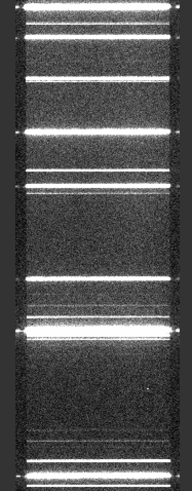
Here is a screen shot of a portion of the arc image as viewed with ginga:
ginga Calibrations/Arc_A_0_DET01.fits
As typical of most arc images, one sees a series of arc lines, here oriented horizontally (as always in PypeIt).
See Arc for further details.
Slit Edges
The code will automatically assign edges to each slit on the detector. For this example, which used the standard long-slit of the Kast instrument, there is only one slit.
Here is a screen shot from the first tab in the ginga window after using the pypeit_chk_edges script, with this explicit call:
pypeit_chk_edges Calibrations/Edges_A_0_DET01.fits.gz
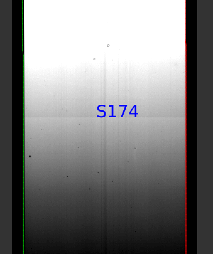
The data is the combined flat images and the green/red lines indicate the left/right slit edges (green/magenta in more recent versions). The S174 label indicates the slit name.
See Edges for further details.
Wavelengths
One should inspect the PypeIt QA for the wavelength
calibration. These are PNGs in the QA/PNG/ folder.
1D
Here is an example of the 1D fits, written to
the QA/PNGs/Arc_1dfit_A_0_DET01_S0175.png file:
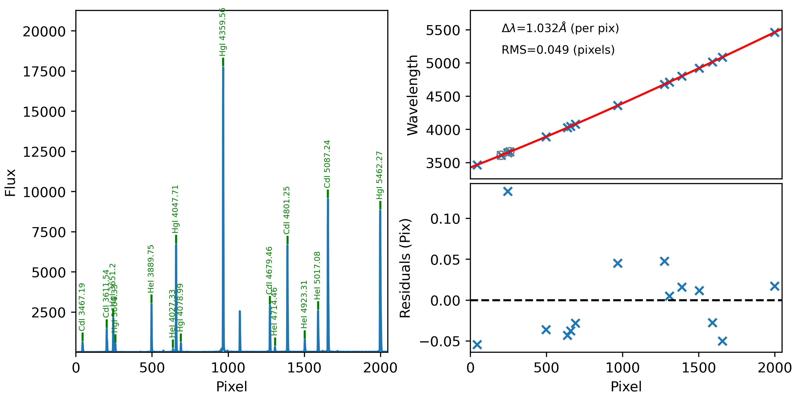
What you hope to see in this QA is:
On the left, many of the blue arc lines marked with green IDs
That the green IDs span the full spectral range.
In the upper right, an RMS < 0.1 pixels
In the lower right, a random scatter about 0 residuals
See WaveCalib for further details.
2D
There are several QA files written for the 2D fits.
Here is QA/PNGs/Arc_tilts_2d_A_0_DET01_S0175.png:
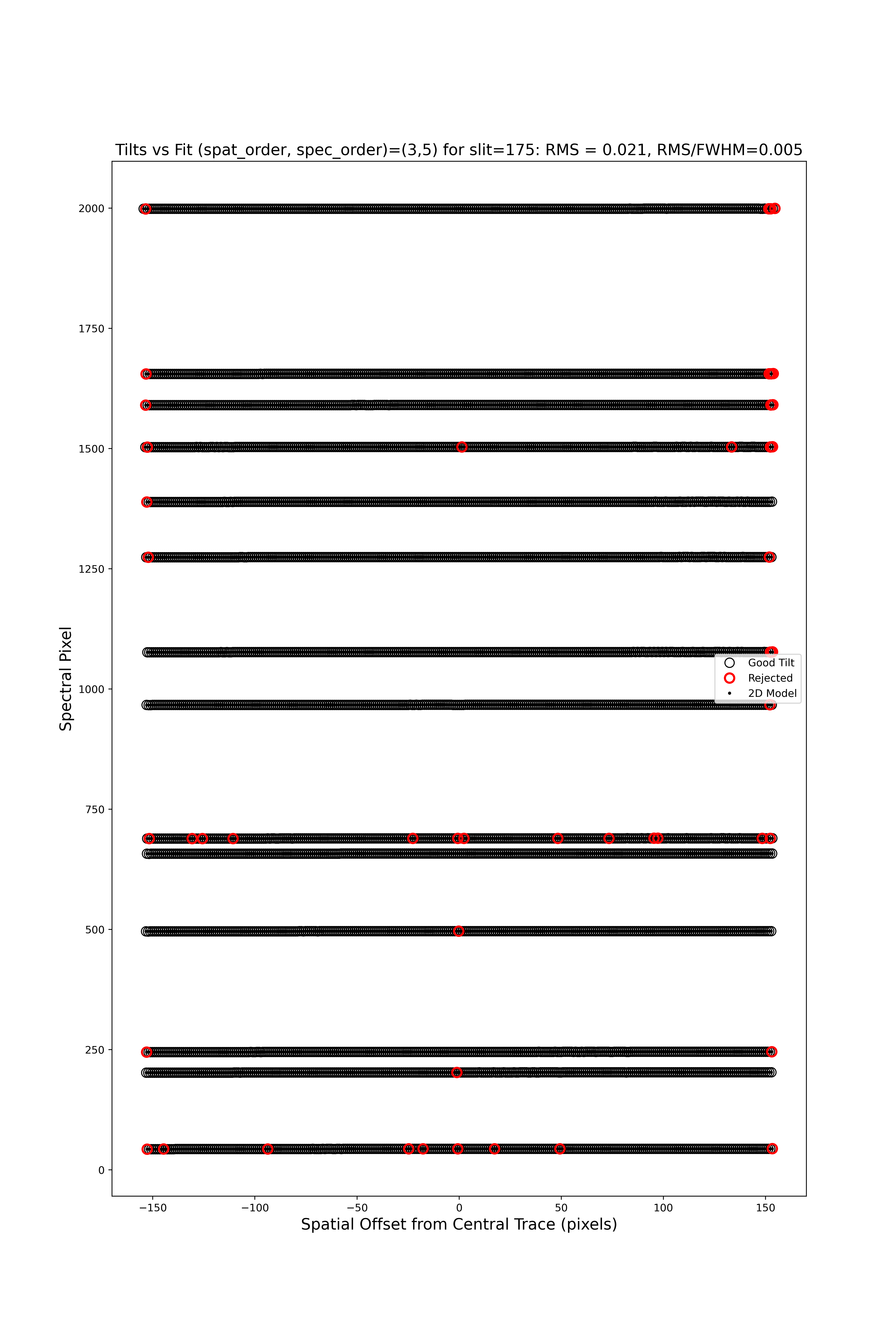
Each horizontal line of circles traces the arc line centroid as a function of spatial position along the slit length. These data are used to fit the tilt in the spectral position. “Good” measurements included in the parametric trace are shown as black points; rejected points are shown in red. Provided most were not rejected, the fit should be good. An RMS<0.1 is also desired.
We also provide a script so that the arcline traces can be assessed against the image using ginga, similar to checking the slit edge tracing.
pypeit_chk_tilts Calibrations/Tilts_A_0_DET01.fits.gz
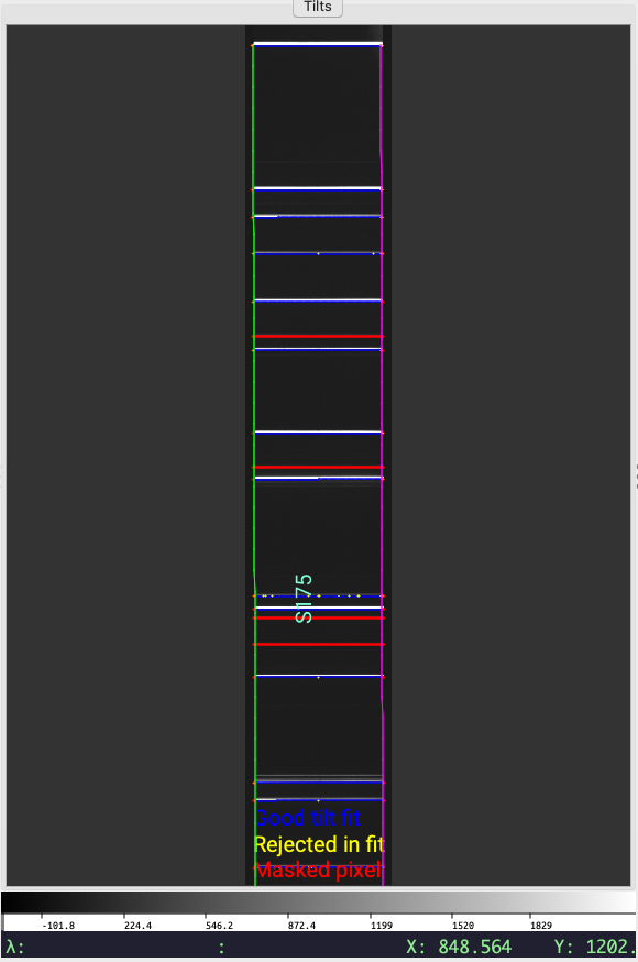
Main ginga window produced by pypeit_chk_tilts. The arc image is
shown in gray scale, the slit edges are shown in green/magenta, masked pixels
are highlighted in red, good centroids are shown in blue, and centroids
rejected during the fit are shown in yellow.
See WaveCalib for further details.
Flatfield
The code produces flat-field images for correcting pixel-to-pixel variations and illumination of the detector.
Here is a screen shot from the first tab in the ginga
window (pixflat_norm) after using
pypeit_chk_flats, with this explicit call:
pypeit_chk_flats Calibrations/Flat_A_0_DET01.fits
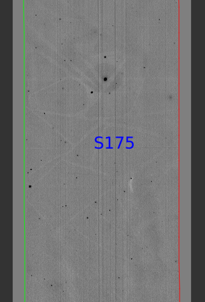
One notes the pixel-to-pixel variations; these are at the percent level. The slit edges defined by the code are also plotted (green/red lines; green/magenta in more recent versions). The region of the detector beyond these images has been set to unity.
See Flat for further details.
Spectra
Eventually (be patient), the code will start generating 2D and 1D spectra
outputs. One per standard and science frame, located in the Science/
folder.
For reference, full processing of this dataset on my circa 2020 Macbook Pro took a little more than 2 minutes.
Spec2D
Here is a screen shot from the third tab in the ginga
window (sky_resid-det01) after using
pypeit_show_2dspec, with this explicit call:
pypeit_show_2dspec Science/spec2d_b27-J1217p3905_KASTb_20150520T045733.560.fits
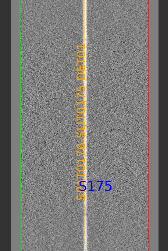
The green/red lines are the slit edges (green/magenta in more recent versions). The brighter pixels down the center of the slit is the object. The orange line shows the PypeIt trace of the object and the orange text is the PypeIt assigned name. The night sky and emission lines have been subtracted.
See Spec2D Output for further details.
Spec1D
Here is a screen shot from the GUI showing the 1D spectrum after using pypeit_show_1dspec, with this explicit call:
pypeit_show_1dspec Science/spec1d_b27-J1217p3905_KASTb_20150520T045733.560.fits
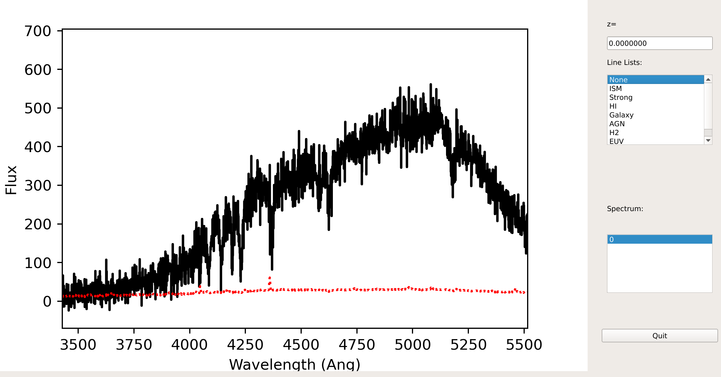
See Spec1D Output for further details.
Fluxing
This dataset includes observations of a spectrophotometric standard, Feige 66, which is reduced alongside the science target observations.
Now that we have a reduced standard star spectrum, we can use that to generate a sensitivity file. Here is the call for this example:
pypeit_sensfunc Science/spec1d_b24-Feige66_KASTb_20150520T041246.960.fits -o Kastb_feige66_sens.fits
This produces the sensitivity function (saved to Kastb_feige66_sens.fits)
and three QA (pdf) plots. The main QA plot looks like this:
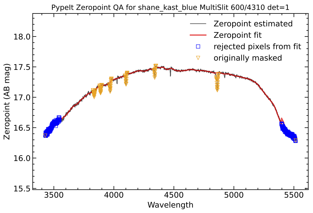
QA plot from the sensitivity calculation. Black is the observed zeropoints, red is the best-fit model, orange are points masked before fitting, blue are points masked during fitting.
The other two plots show the flux-calibrated standard-star spectrum against the archived spectrum and the full system (top of atmosphere) throughput.
See Fluxing for further details.