Coadd2D HOWTO
Overview
This document explains how to run pypeit_coadd_2dspec, including three examples using multi-slit observations:
When Running the Script
pypeit_coadd_2dspec is run only after a successful main reduction (i.e., run_pypeit). See Tutorials for example executions of run_pypeit for a subset of instruments.
Coadd2d File
pypeit_coadd_2dspec requires an input file to guide the process, called
the coadd2d file (see coadd2d file). Similar to pypeit_setup,
we provide a script that can be used to automatically generate one or more
coadd2d files for you; see here. Although
this script will at least get you started with the coadd2d file, you may
need to edit the file to ensure the coadding is performed as you desire. Here,
we further explain the format of the file and some typical edits you might want
to make.
The format of the coadd2d Input File includes a
Parameter Block (optional) and a Data Block (required).
Here is an example coadd2d file:
# User-defined execution parameters
[rdx]
    spectrograph = keck_mosfire
[reduce]
    [[findobj]]
        snr_thresh=5.0
[coadd2d]
    offsets = maskdef_offsets
    weights = uniform
    manual = 1:22.4:608.1:3.,2:22.4:608.1:3.       # det:spat:spec:fwhm

# Data block
spec2d read
filename
Science/spec2d_MF.20180718.22100-HIP61138_MOSFIRE_20180718T060820.621.fits
Science/spec2d_MF.20180718.22154-HIP61138_MOSFIRE_20180718T060914.170.fits
spec2d end
Data Block
The data block includes a list of reduced 2D spectra files, which can be found in the Science
folder:
$ ls -1 Science/spec2d*.fits
Science/spec2d_MF.20180718.22100-HIP61138_MOSFIRE_20180718T060820.621.fits
Science/spec2d_MF.20180718.22154-HIP61138_MOSFIRE_20180718T060914.170.fits
Parameter Block
The parameter block includes the parameters used to guide the 2D coadding and the reduction (i.e., object finding and extraction) of the coadded spectra. The parameters for the reduction are the same as the ones used during the main PypeIt run, see ReducePar Keywords. For the full set of 2D coadding parameters, see Coadd2DPar Keywords. We highlight a few parameters below.
manual
The coadd2d parameter manual provides the location of the objects that the user want to manually extract.
Each object location is separated by a semi-colon and is constructed as det:spat:spec:fwhm, which means
that the object is located in detector det at the spatial pixel spat and spectral pixel spec
and it has a FWHM equal to fwhm. The location of the object must be in the 2D coadded frame, therefore
pypeit_coadd_2dspec must be run twice: once to inspect the 2D coadded frame and locate the object,
and a second time to perform the manual extraction. See Manual Extraction.
offsets
This parameter defines the offsets in spatial pixels between the frames to be coadded. Here are the options:
offsets = auto: PypeIt will compute the offsets. If the parameteruser_obj_ids(see Coadd2DPar Keywords) is also set, PypeIt will use the 1D extracted spectrum chosen by the user to compute the offsets, otherwise it will use the 1D extracted spectrum with the highest S/N. If such spectrum is not found in each frame that the user wants to coadd, PypeIt will stop with an error. In this case a list of offsets should be provided, or setoffsets = maskdef_offsetsif available. This is the default.offsetsis alist(e.g.,offsets = 0.,1.2,-2.5): These values will be used as they are.offsets = maskdef_offsets: PypeIt will use the offsets, determined during the main reduction run, between the position of the extracted objects and their expected position from the slitmask design information.offsets = header: PypeIt will use the dither offsets recorded in the header, if available.
Note
The offsets = maskdef_offsets option is only available for multi-slit observations and
currently only for these Slit-mask design Spectrographs.
Set the parameters SlitMaskPar Keywords in the PypeIt Reduction File during
the main PypeIt run to determine how maskdef_offsets are computed. See RA, Dec and object name assignment to 1D extracted spectra
for more info.
weights
This parameter defines the weights to be used in the 2D coadding.
weights = auto: PypeIt will try to compute the (S/N)^2 weights. If the parameteruser_obj_ids(see Coadd2DPar Keywords) is also set, PypeIt will use the 1D extracted spectrum chosen by the user to compute the weights, otherwise it will use the 1D extracted spectrum with the highest S/N. If such spectrum is not found in each frame that the user wants to coadd, PypeIt will use uniform weights. This is the default.weightsis alist(e.g.,weights = 1.,1.,1.): These values will be used as they are.weights = uniform: PypeIt will use uniform weights.
Keck/LRIS Example
LRIS: Create coadd2D file
Using the keck_lris_blue/multi_600_4000_d560 dataset from the
PypeIt Development Suite as an example, a successful execution of run_pypeit using the
keck_lris_blue_multi_600_4000_d560.pypeit should result in the following spec2d files:
$ ls -1 Science/spec2d*.fits
Science/spec2d_b170320_2083-c17_60L._LRISb_20170320T055336.211.fits
Science/spec2d_b170320_2090-c17_60L._LRISb_20170320T082144.525.fits
Science/spec2d_b170320_2084-c17_60L._LRISb_20170320T062414.630.fits
Science/spec2d_b170320_2091-c17_60L._LRISb_20170320T085223.894.fits
You can automatically generate the coadd2d script by executing
pypeit_setup_coadd2d -f keck_lris_blue_multi_600_4000_d560.pypeit --only_slits 30 70 111 156 216 --det 2
The --only_slits option allows you to specify specific slits to coadd,
instead of coadding all that are available. We also select to only combine the
data on detector 2. The result of the script is a file called
keck_lris_blue_multi_600_4000_d560_c17_60L..coadd2d, which looks like this:
# Auto-generated Coadd2D input file using PypeIt version: 1.12.3.dev337+g096680b06.d20230503
# UTC 2023-05-08T19:45:26.885

# User-defined execution parameters
[rdx]
    spectrograph = keck_lris_blue
    redux_path = /path/to/PypeIt-development-suite/REDUX_OUT/keck_lris_blue/multi_600_4000_d560
    scidir = Science
    qadir = QA
    detnum = 2,
[calibrations]
    calib_dir = Calibrations
    [[wavelengths]]
        refframe = observed
[coadd2d]
    offsets = auto
    weights = auto
    only_slits = 30, 70, 111, 156, 216
[flexure]
    spec_method = skip
[reduce]
    [[findobj]]
        skip_skysub = True

# Data block
spec2d read
 path /path/to/PypeIt-development-suite/REDUX_OUT/keck_lris_blue/multi_600_4000_d560/Science
                                                   filename
spec2d_b170320_2083-c17_60L._LRISb_20170320T055336.211.fits
spec2d_b170320_2084-c17_60L._LRISb_20170320T062414.630.fits
spec2d_b170320_2090-c17_60L._LRISb_20170320T082144.525.fits
spec2d_b170320_2091-c17_60L._LRISb_20170320T085223.894.fits
spec2d end
Note that the default Coadd2DPar Keywords parameters are set to offsets = auto
and weights = auto. See Setup script for additional parameters.
Note
The Setup script script is new as of version 1.13.0. Some of
the options that were passed to pypeit_coadd2d in previous versions are
now passed to pyepit_setup_coadd2d instead. One example is the use of
--only_slits above; another is that objects are selected in
pypeit_setup_coadd2d, not pypeit_coadd_2dspec.
LRIS: Run
Once the coadd2d file is ready, the main call is simply:
$ pypeit_coadd_2dspec keck_lris_blue_multi_600_4000_d560_c17_60L..coadd2d
At the beginning of the run, the user should inspect the information printed on the terminal by the script, and verify that the offsets and the way the weights are computed are accepted. This is an example of the information printed on the terminal:
[INFO]    :: Get Weights
[INFO]    :: Weights computed using a unique reference object in slit=582 with the highest S/N
[INFO]    ::
             -------------------------------------
               Summary for highest S/N object
                   found on slitid = 582
             -------------------------------------
                        exp#        S/N
                         0          5.44
                         1          4.31
                         2          5.64
                         3          5.21
             -------------------------------------
[INFO]    :: Get Offsets
[INFO]    :: Determining offsets using brightest object found on slit: 582 with avg SNR= 5.15
(...)
             ---------------------------------------------
              Summary of offsets from brightest object found on slit: 582 with avg SNR= 5.15
             ---------------------------------------------
                        exp#      offset
                         0         0.00
                         1         0.13
                         2         0.24
                         3        -0.04
             -----------------------------------------------
This confirms that both weights and offsets are computed using an object with the highest S/N and shows the report on what was found.
LRIS: Output
At the end of the run the code will generate 2D and 1D spectra outputs located in the
Science_coadd/ folder. These outputs are identical to the ones generated by the main PypeIt
reduction.
LRIS: Inspecting spec2d output
Here is a screen shot from the third tab in the ginga window (sky_resid-DET02) after using pypeit_show_2dspec, with this explicit call:
$ pypeit_show_2dspec Science_coadd/spec2d_b170320_2083-b170320_2091-c17_60L..fits --det DET02
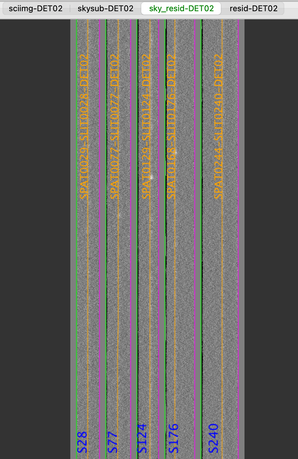
The green/magenta lines are the slit edges. The orange line shows the PypeIt trace of the object and the orange text is the PypeIt assigned name.
See Spec2D Output for further details.
LRIS: Inspecting spec1d output
Like for the main PypeIt reduction, a summary of all the extracted sources can be
found in the Science_coadd/spec1d_b170320_2083-b170320_2091-c17_60L..txt file. Here is an
example of how it looks:
| slit |                    name | spat_pixpos | spat_fracpos | box_width | opt_fwhm |  s2n |
|   28 | SPAT0029-SLIT0028-DET02 |        28.7 |        0.492 |      3.00 |    1.392 | 0.85 |
|   77 | SPAT0077-SLIT0077-DET02 |        77.0 |        0.501 |      3.00 |    1.030 | 0.76 |
|  124 | SPAT0129-SLIT0124-DET02 |       128.7 |        0.608 |      3.00 |    1.325 | 1.90 |
|  176 | SPAT0168-SLIT0176-DET02 |       168.4 |        0.331 |      3.00 |    1.145 | 1.20 |
|  240 | SPAT0244-SLIT0240-DET02 |       244.2 |        0.563 |      3.00 |    1.045 | 0.87 |
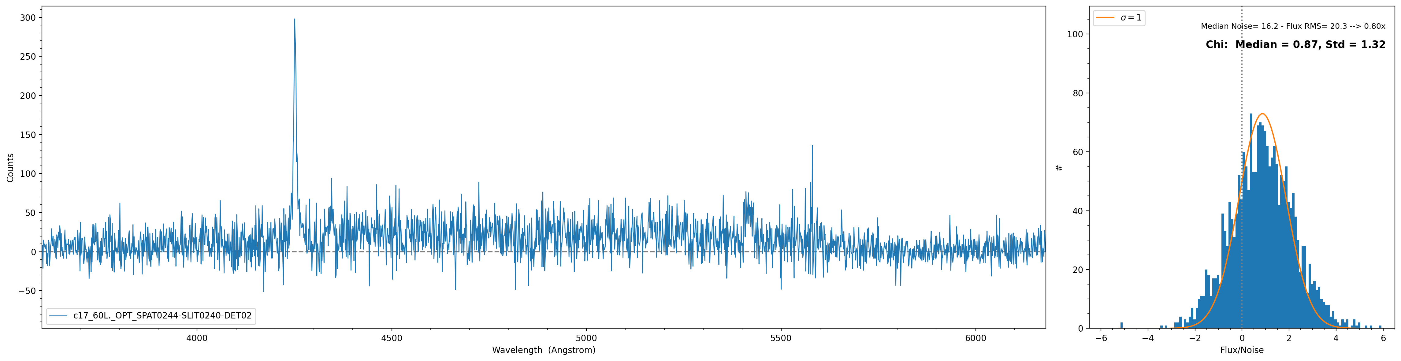
The spec1d can also be inspected with the script pypeit_chk_noise_1dspec, which show the spec1D for
visual inspection and a noise diagnostic plot. Here is an example of the call and how the plots looks:
$ pypeit_chk_noise_1dspec Science_coadd/spec1d_b170320-b170320-c17.fits --pypeit_name SPAT0244-SLIT0240-DET02
Warning
The exact name of the object may change due to slight spatial shifts in where the object is found.
The plot on the right is showing the distribution of Flux/Noise of the extracted spectrum. In this example
there is clearly flux coming from the object that biases the Flux/Noise diagnostic plot. However, this script
provides the possibility to select a region in the spectrum without emission to be used for the diagnostic plot.
The script usage can be displayed by calling the script with the
-h option:
$ pypeit_chk_noise_1dspec -h
usage: pypeit_chk_noise_1dspec [-h] [-v VERBOSITY] [--log_file LOG_FILE]
                               [--log_level LOG_LEVEL] [--fileformat FILEFORMAT]
                               [--extraction EXTRACTION] [--ploterr] [--step]
                               [--z [Z ...]] [--maskdef_objname MASKDEF_OBJNAME]
                               [--pypeit_name PYPEIT_NAME] [--wavemin WAVEMIN]
                               [--wavemax WAVEMAX] [--plot_or_save PLOT_OR_SAVE]
                               [--try_old]
                               [files ...]

Examine the noise in a PypeIt spectrum

positional arguments:
  files                 PypeIt spec1d file(s) (default: None)

options:
  -h, --help            show this help message and exit
  -v, --verbosity VERBOSITY
                        Verbosity level, which must be 0, 1, or 2. Level 0
                        includes warning and error messages, level 1 adds
                        informational messages, and level 2 adds debugging
                        messages and the calling sequence. (default: 2)
  --log_file LOG_FILE   Name for the log file. If set to "default", a default
                        name is used. If None, a log file is not produced.
                        (default: None)
  --log_level LOG_LEVEL
                        Verbosity level for the log file. If a log file is
                        produce and this is None, the file log will match the
                        console stream log. (default: None)
  --fileformat FILEFORMAT
                        Is this coadd1d or spec1d? (default: spec1d)
  --extraction EXTRACTION
                        If spec1d, which extraction? opt or box (default: opt)
  --ploterr             Plot noise spectrum (default: False)
  --step                Use `steps-mid` as linestyle (default: False)
  --z [Z ...]           Object redshift (default: None)
  --maskdef_objname MASKDEF_OBJNAME
                        MASKDEF_OBJNAME of the target that you want to plot. If
                        maskdef_objname is not provided, nor a pypeit_name, all
                        the 1D spectra in the file(s) will be plotted. (default:
                        None)
  --pypeit_name PYPEIT_NAME
                        PypeIt name of the target that you want to plot. If
                        pypeit_name is not provided, nor a maskdef_objname, all
                        the 1D spectra in the file(s) will be plotted. (default:
                        None)
  --wavemin WAVEMIN     Wavelength min. This is for selecting a region of the
                        spectrum to analyze. (default: None)
  --wavemax WAVEMAX     Wavelength max.This is for selecting a region of the
                        spectrum to analyze. (default: None)
  --plot_or_save PLOT_OR_SAVE
                        Do you want to save to disk or open a plot in a mpl
                        window. If you choose save, a folder called
                        spec1d*_noisecheck will be created and all the relevant
                        plot will be placed there. (default: plot)
  --try_old             Attempt to load old datamodel versions. A crash may
                        ensue.. (default: False)
Keck/DEIMOS Example
DEIMOS: Create coadd2D file
After a successful reduction with run_pypeit, we create a coadd 2D file.
Our coadd2d file is called keck_deimos_1200g_m_7750_dra11.coadd2d and looks like this:
# User-defined execution parameters
[rdx]
    spectrograph = keck_deimos
    detnum = 7
[reduce]
    [[findobj]]
        snr_thresh = 10.0
[coadd2d]
    offsets = maskdef_offsets
    weights = auto
    user_obj_ids = 1032, 1032, 1031

# Data block
spec2d read
filename
Science/spec2d_DE.20170425.50487-dra11_DEIMOS_20170425T140121.014.fits
Science/spec2d_DE.20170425.51771-dra11_DEIMOS_20170425T142245.350.fits
Science/spec2d_DE.20170425.53065-dra11_DEIMOS_20170425T144418.240.fits
spec2d end
In this example we 2D coadd only one detector (det 7); however, note that PypeIt
uses, as default, a mosaic approach for the reduction of Keck/DEIMOS, for which a mosaic
is constructed for each blue-red detector pair. See Keck DEIMOS for more detail.
Because weights = auto, the parameter user_obj_ids in this example instructs PypeIt
to use the 1D extracted spectrum with unique object identifier equal to 1032 in the first frame,
1032 in the second frame, and 1031 in the third frame, to compute the weights. Each value of
user_obj_ids can be found in the spec1d*.txt file (under obj_id) and corresponds to
the SPAT_PIXPOS_ID or ECH_FRACPOS_ID attribute (for slit or echelle spectroscopy, respectively)
of the spec1d object. See Spec1D Output for more info about SPAT_PIXPOS_ID and ECH_FRACPOS_ID.
Note
As you can see we set offsets = maskdef_offsets. For this DEIMOS dataset we computed the
maskdef_offsets in the main PypeIt reduction by using these parameters in the PypeIt Reduction File:
[reduce]
    [[slitmask]]
        use_alignbox = True
which means that the offsets have been computed using the stars in the alignment boxes.
DEIMOS: Run
Once the coadd2d file is ready, the main call is simply:
$ pypeit_coadd_2dspec keck_deimos_1200g_m_7750.coadd2d
The script will print in the terminal something like this:
[INFO]    :: Get Weights
[INFO]    :: Weights computed using a unique reference object in slit=1037 provided by the user
[INFO]    :: Get Offsets
[INFO]    :: Determining offsets using maskdef_offset recoded in SlitTraceSet
[INFO]    ::
             ---------------------------------------------
              Summary of offsets from maskdef_offset
             ---------------------------------------------
                        exp#      offset
                         0         0.00
                         1         0.24
                         2         0.96
             -----------------------------------------------
This confirms our choice for how to compute weights and offsets and shows the report on what was found.
DEIMOS: Inspecting spec2d output
Here is a screen shot from the third tab in the ginga`_ window (sky_resid-DET07) after using pypeit_show_2dspec, with this explicit call:
$ pypeit_show_2dspec Science_coadd/spec2d_DE.20170425.50487-DE.20170425.53065-dra11.fits --det DET07
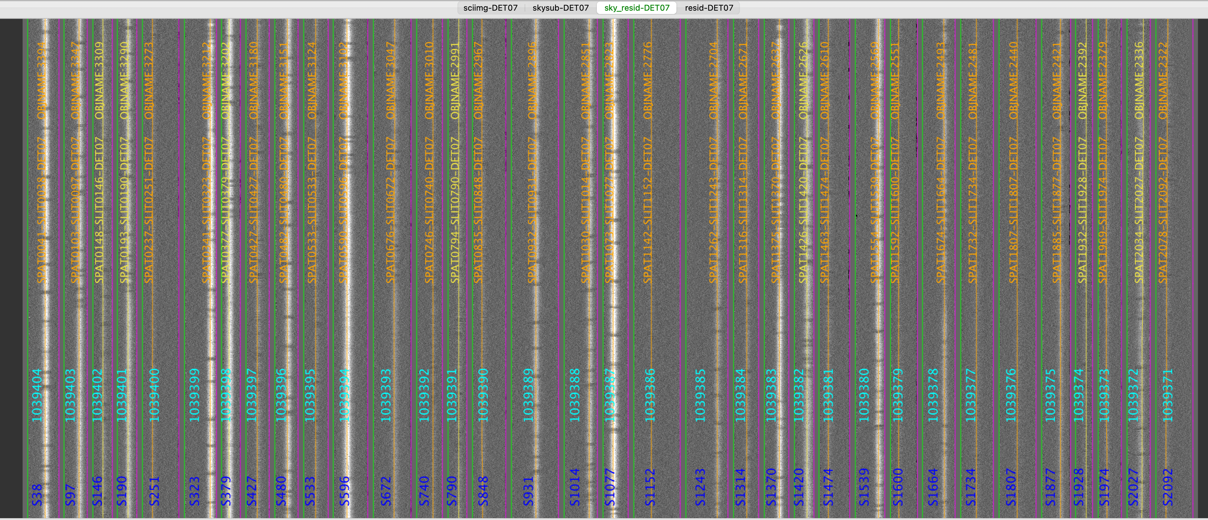
The green/magenta lines are the slit edges. The orange line shows the PypeIt trace of the object and the orange text is the PypeIt assigned name plus the object name from the slitmask design. Yellow lines and text indicate sources that had insufficient S/N for detection, but were force extracted using the information in the slitmask design.
See Spec2D Output for further details.
DEIMOS: Inspecting spec1d output
A summary of all the extracted sources can be found in the spec1d_DE.20170425.50487-DE.20170425.53065-dra11.txt
file in the Science_coadd/ folder. See Spec1D for an example of this file with the
explanation for some columns.
The spec1d can also be inspected with the script pypeit_chk_noise_1dspec, which show the spec1D for
visual inspection and a noise diagnostic plot. See example in LRIS: Inspecting spec1d output.
Keck/MOSFIRE Example
MOSFIRE: Create coadd2D file
After a successful reduction with run_pypeit, we create a coadd 2D file.
Our coadd2d file is called keck_mosfire.coadd2d and looks like this:
[rdx]
    spectrograph = keck_mosfire
[coadd2d]
    offsets = maskdef_offsets
    weights = auto
    only_slits = 1987, 721, 410, 151

# Data block
spec2d read
filename
Science/spec2d_m120910_0163-MOSFIRE_DRP_MAS_MOSFIRE_20120910T123447.585.fits
Science/spec2d_m120910_0164-MOSFIRE_DRP_MAS_MOSFIRE_20120910T123537.585.fits
spec2d end
Note
For this MOSFIRE dataset we computed the maskdef_offsets in the main PypeIt reduction
by using these parameters in the PypeIt Reduction File:
[reduce]
    [[slitmask]]
        use_dither_offset = False
        bright_maskdef_id = 1
which means that the offsets have been computed using a bright object in the slit with Slit_Number=1.
MOSFIRE: Run
Once the coadd2d file is ready, the main call is simply:
$ pypeit_coadd_2dspec keck_mosfire.coadd2d
The script will print in the terminal something like this:
[INFO]    :: Get Weights
[INFO]    :: Weights computed using a unique reference object in slit=151 with the highest S/N
[INFO]    ::
             -------------------------------------
               Summary for highest S/N object
                   found on slitid = 151
             -------------------------------------
                        exp#        S/N
                         0         18.77
                         1         19.36
             -------------------------------------

[INFO]    :: Get Offsets
[INFO]    :: Determining offsets using maskdef_offset recoded in SlitTraceSet
[INFO]    ::
             ---------------------------------------------
              Summary of offsets from maskdef_offset
             ---------------------------------------------
                        exp#      offset
                         0         0.00
                         1        -27.81
             -----------------------------------------------
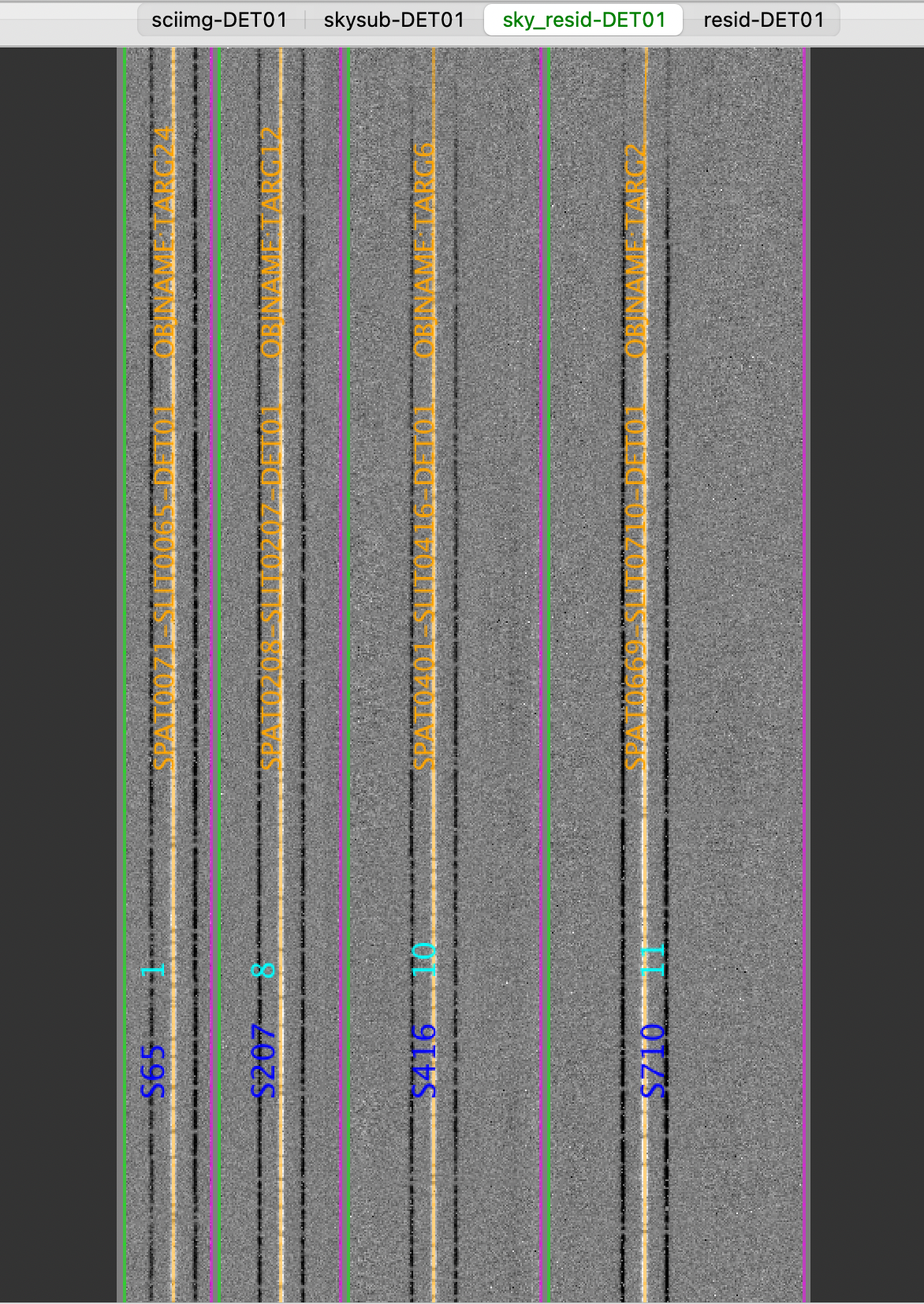
MOSFIRE: Inspecting spec2d output
Here is a screen shot from the third tab in the ginga window (sky_resid-DET01) after using pypeit_show_2dspec, with this explicit call:
$ pypeit_show_2dspec Science_coadd/spec2d_m120910-m120910-MOSFIRE.fits
MOSFIRE: Inspecting spec1d output
A summary of all the extracted sources can be found in the spec1d_m120910-m120910-MOSFIRE.txt file
in the Science_coadd/ folder. Here is an example:
| slit |                    name | maskdef_id | objname |     objra |   objdec | spat_pixpos | spat_fracpos | box_width | opt_fwhm |   s2n | maskdef_extract |
|   65 | SPAT0071-SLIT0065-DET01 |          1 |  TARG24 | 344.92242 | 33.00392 |        70.9 |        0.549 |      3.00 |    0.730 | 19.25 |           False |
|  207 | SPAT0208-SLIT0207-DET01 |          8 |  TARG12 | 345.00158 | 33.00703 |       207.7 |        0.501 |      3.00 |    0.630 | 22.81 |           False |
|  416 | SPAT0401-SLIT0416-DET01 |         10 |   TARG6 | 345.02304 | 33.01136 |       401.2 |        0.437 |      3.00 |    0.640 | 18.35 |           False |
|  710 | SPAT0669-SLIT0710-DET01 |         11 |   TARG2 | 345.04113 | 33.01283 |       668.7 |        0.373 |      3.00 |    0.656 | 28.52 |           False |
The spec1d can also be inspected with the script pypeit_chk_noise_1dspec, which show the spec1D for
visual inspection and a noise diagnostic plot. See example in LRIS: Inspecting spec1d output.