SOAR/TripleSpec HOWTO
Overview
This doc goes through a full run of PypeIt on an example SOAR/TripleSpec dataset (a reduction of the transient 2025cy with its A0 V telluric standard HD 116699). TripleSpec is a fixed-format, cross-dispersed near-infrared spectrograph; PypeIt reduces it with the Echelle pipeline over five orders (order numbers 7 through 3), covering roughly 0.8–2.47 microns. If you’re having trouble reducing your data, we encourage you to work through this tutorial first. See also the instrument notes at SOAR TripleSpec, join our PypeIt Users Slack using this invitation link to ask for help, and/or Submit an issue to GitHub if you find a bug!
Setup
Before reducing your data with PypeIt, you first have to prepare a PypeIt Reduction File by running pypeit_setup:
pypeit_setup -r /path/to/raw/ -s soar_tspec -b -c A
where the -r argument should be replaced by your local raw-data directory
and -b indicates that the data use background (sky) subtraction and the
calib, comb_id, and bkg_id columns should be added to the
Data Block. TripleSpec has a single fixed configuration, so -c A
and -c all are equivalent.
This produces a directory soar_tspec_A containing the pypeit file
soar_tspec_A.pypeit. The key part is the Data Block, which for this
example looks like:
# Data block
data read
 path ./
                                filename |        frametype | ... | dispname | binning | exptime | calib | comb_id | bkg_id
#          SPEC_ARC_04-02-2025_0103.fits |         arc,tilt | ... |     spec |     1,1 |     2.0 |     0 |      -1 |     -1
         SPEC_DFLAT_04-02-2025_0088.fits |             dark | ... |     spec |     1,1 |     2.0 |     0 |      -1 |     -1
         SPEC_DFLAT_04-02-2025_0042.fits |  pixelflat,trace | ... |     spec |     1,1 |     2.0 |     0 |      -1 |     -1
        SPEC_2025cy_05-02-2025_0116.fits | arc,tilt,science | ... |     spec |     1,1 |   300.0 |     0 |       1 |      2
        SPEC_2025cy_05-02-2025_0117.fits | arc,tilt,science | ... |     spec |     1,1 |   300.0 |     0 |       2 |      1
SPEC_2025cy_05-02-2025_standard0120.fits |         standard | ... |     spec |     1,1 |    9.25 |     0 |       3 |      4
SPEC_2025cy_05-02-2025_standard0121.fits |         standard | ... |     spec |     1,1 |    9.25 |     0 |       4 |      3
data end
Wavelength-calibration frames
Note that the science frames are typed arc,tilt,science. This is the most
important edit to make for TripleSpec: there is no arc lamp that is useful
across the full near-IR range, so the dense forest of OH sky-emission lines in
the science frames is used as the wavelength reference. The short dedicated arc
exposure (SPEC_ARC_...) is therefore commented out. The 300 s science
exposures have far more usable OH signal than a short arc, especially in the
reddest order.
The standard-star frames are not typed as arc,tilt because the short
(9.25 s) standard exposures do not contain enough OH signal for a good
solution. Instead, by giving the standards the same calib value as the
science frames, PypeIt applies the science-derived wavelength solution to them.
Warning
If you change the frame typing (e.g. which frames serve as the arc), you
must delete the affected files in Calibrations/ before re-running.
run_pypeit -o overwrites only the science products, not the cached
calibration frames, so a stale Arc_* / WaveCalib_* would silently be
reused and yield a confusing failure.
A-B differencing
The comb_id and bkg_id columns implement A-B sky subtraction for the
ABBA dither sequence. For the science pair, frame 0116 has comb_id=1,
bkg_id=2 (treat as A, subtract B) and frame 0117 reverses them (treat as
B, subtract A); the standard pair is handled the same way. PypeIt builds the
A-B and B-A images, whose positive residuals are the source flux, and these can
later be combined with 2D coadding. See
A-B image differencing for the full description.
Core Processing
To perform the core processing, run run_pypeit:
run_pypeit soar_tspec_A.pypeit
The code runs uninterrupted through order tracing, wavelength calibration, field flattening, object finding, sky subtraction, and spectral extraction; see PypeIt’s Core Data Reduction Executable and Workflow. As it runs it produces a number of files and QA plots to inspect.
Order Edges
The code first uses the trace frames (dome flats with the lamp on) to find
the order edges. TripleSpec is a fixed-format echelle, so the trace should
always look the same: five orders. Inspect them with:
pypeit_chk_edges Calibrations/Edges_A_0_DET01.fits.gz
This opens a ginga window with the trace image overlaid (green = left edge, magenta = right edge). PypeIt expects to find all 5 orders and will fault if it does not.
Tip
The default parameters disable the order PCA (auto_pca = False) and use
direct polynomial fits to the order edges, which are robust for this
detector. If edge tracing misbehaves on your data, see the User-level Parameters
and specifically the EdgeTracePar Keywords.
Wavelength Calibration
Next the code performs the wavelength calibration from the OH sky lines, using
the reidentify method against the bundled soar_triplespec.fits archive
and the OH_NIRES line list (see SOAR TSPEC (soar_tspec)).
Check the per-order result with the automatically generated 1D-fit QA. Below is the plot for the reddest order (order = 3, K band), the most challenging one:
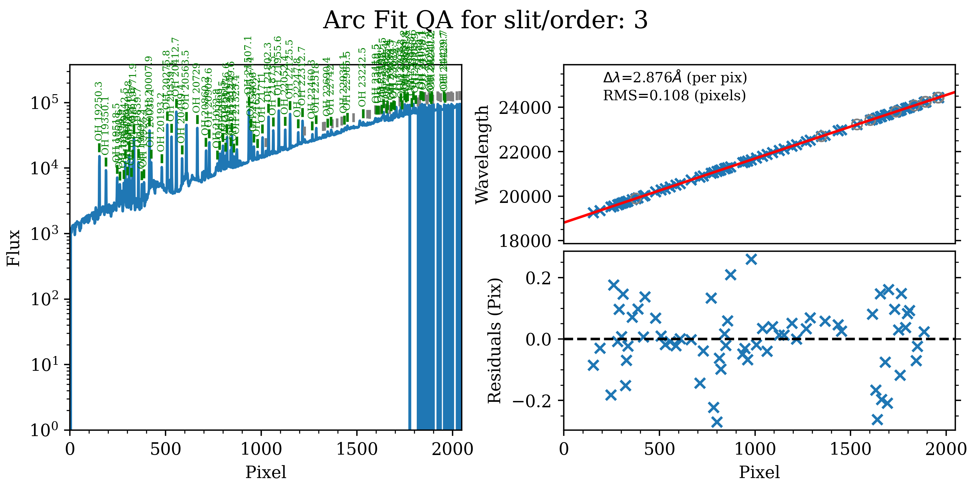
The 1D wavelength-calibration QA for the reddest SOAR/TripleSpec order
(order = 3), Arc_1dfit_A_0_DET01_S0003.png. The left panel is the OH-sky
arc spectrum extracted down the center of the order; green marks lines used in
the solution and gray marks detected features that were not used. The
top-right panel shows the fit (red) to wavelength vs. spectral pixel (blue);
the bottom-right panel shows the residuals. The RMS here is ~0.11 pixels.
The script pypeit_chk_wavecalib summarizes all orders:
pypeit_chk_wavecalib Calibrations/WaveCalib_A_0_DET01.fits
which prints:
 N. SpatOrderID minWave Wave_cen maxWave dWave Nlin     IDs_Wave_range    IDs_Wave_cov(%) measured_fwhm  RMS
--- ----------- ------- -------- ------- ----- ---- --------------------- --------------- ------------- -----
  0           7  8106.5   9389.6 10644.7 1.242   47  9442.240 - 10588.762            45.2           2.1 0.099
  1           6  9450.3  10937.7 12399.6 1.444   91  9793.676 - 12351.597            86.7           2.2 0.070
  2           5 11324.4  13104.7 14857.2 1.730   85 11354.191 - 14833.093            98.5           2.2 0.105
  3           4 14133.8  16354.3 18543.8 2.159   90 14163.034 - 18459.584            97.4           2.3 0.065
  4           3 18806.4  21760.6 24681.4 2.876   68 19250.306 - 24220.763            84.6           2.2 0.108
All five orders are solved with RMS ~0.07–0.11 pixels, spanning ~8100–24700 Angstrom. See pypeit_chk_wavecalib for a description of the columns.
Warning
A common failure mode for sky-line wavelength calibration is that the on-sky exposures are too short to give good OH signal in all orders. When observing, ensure at least some science exposures are long enough. The reddest order (order 3) is the first to suffer.
PypeIt then traces each sky line across the spatial direction of each order to build the 2D wavelength solution. The global QA plot is:
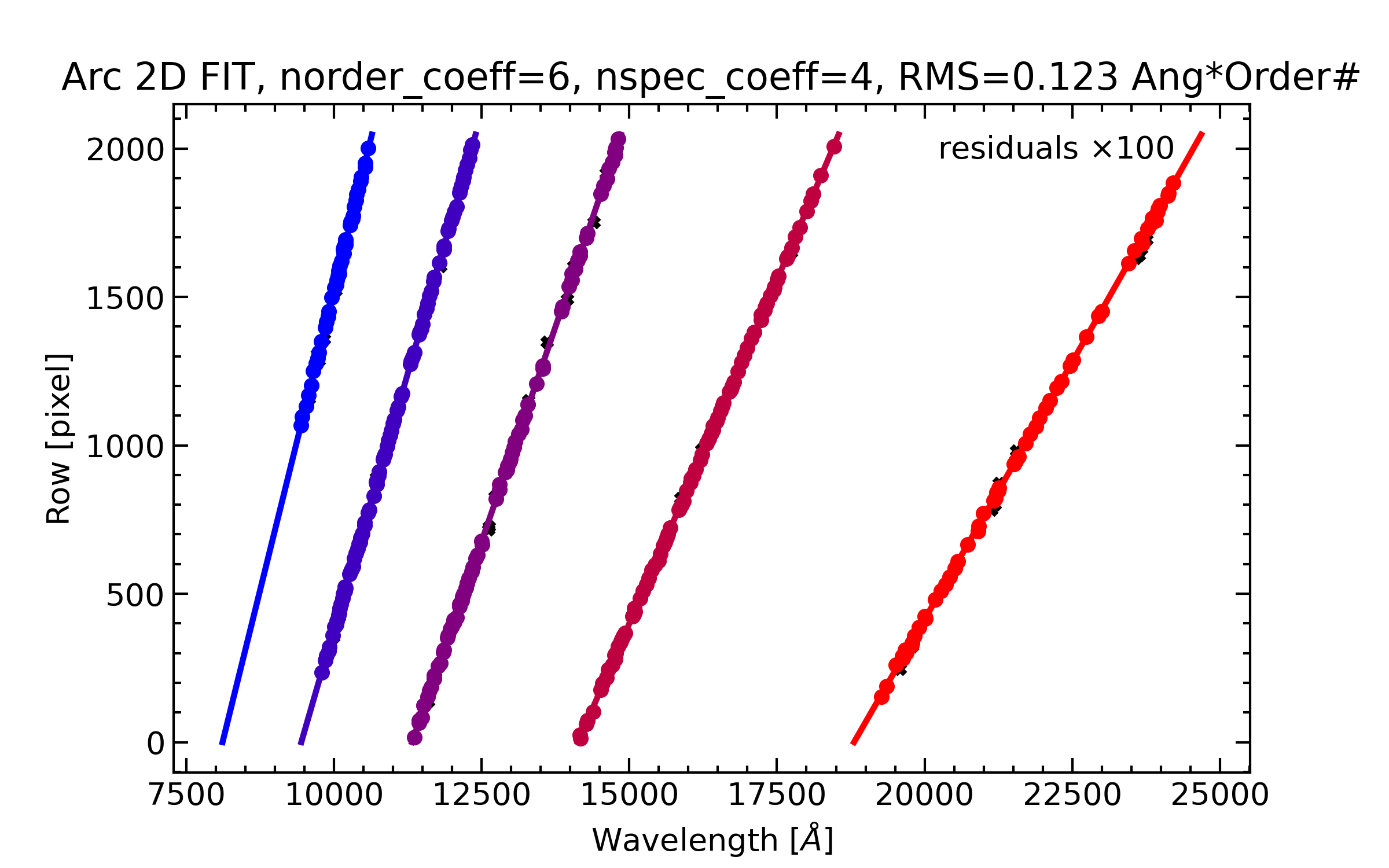
The global 2D wavelength solution, Arc_2dfit_global_A_0_DET01.png,
showing all five orders (colored points) as row vs. wavelength, with the
overall fit RMS quoted at the top.
A per-order 2D tilt QA is also produced:
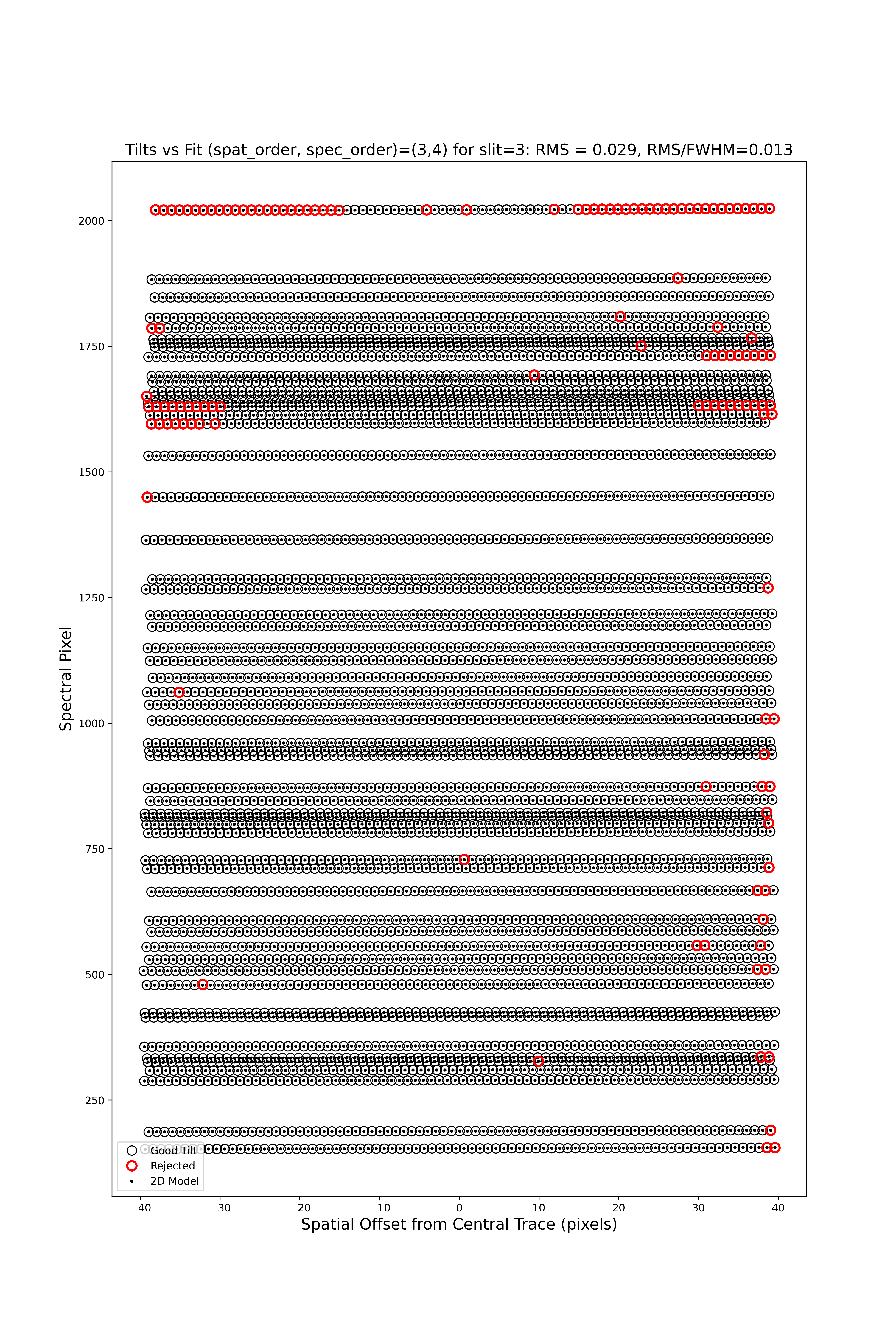
The 2D tilt QA for order 3, Arc_tilts_2d_A_0_DET01_S0003.png. Open
circles are measured sky-line centers (black = kept, red = rejected); the
modeled positions are overlaid.
Field Flattening
PypeIt applies pixel-to-pixel and illumination flat-field corrections built from
the dome flats; the lamp-off dome flats (typed dark) are subtracted first to
remove the thermal/dome background. Inspect them with:
pypeit_chk_flats Calibrations/Flat_A_0_DET01.fits
Object Finding and Extraction
After the calibrations, PypeIt identifies sources, performs global and local sky subtraction, and extracts 1D spectra; see Object Finding. Here is the object-finding QA for the science target in order 7:
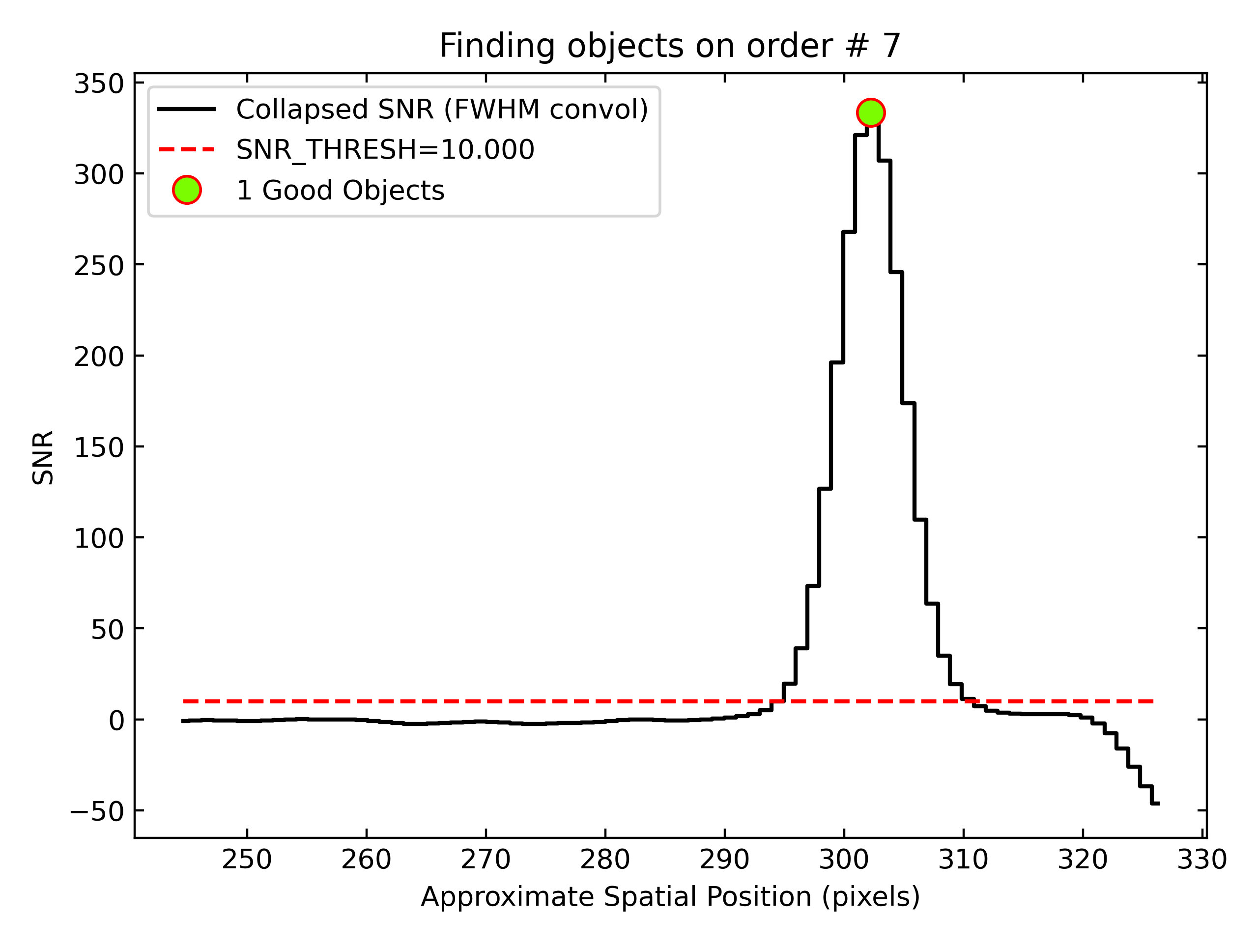
Detection of the 2025cy spectrum in order 7. The black line is the spectrally collapsed S/N as a function of spatial position; the dashed red line is the S/N threshold (set by the FindObjPar Keywords), and the green circle marks the detected object at S/N ~ 28 (rising to ~30 in the bluer orders).
Core Processing Outputs
The primary outputs are calibrated 2D spectral images and 1D extractions; see Outputs.
2D Spectral Images
Each combination group produces a spec2d file. Inspect it with
pypeit_show_2dspec:
pypeit_show_2dspec Science/spec2d_SPEC_2025cy_05-02-2025_0116-2025cy_TSPEC_20250205T040918.237.fits --removetrace
The --removetrace option is useful for faint sources. Check that the object
is well traced in the sciimg channel, that there are minimal sky residuals
in the sky_resid channel, and that the resid channel looks like pure
noise (see also pypeit_chk_noise_2dspec).
1D Spectral Extractions
Each combination group also produces a spec1d fits file plus a .txt
summary. For the standard star HD 116699 (frame 0120) the summary is:
| order |          name | spat_pixpos | spat_fracpos | box_width | opt_fwhm |    s2n | wv_rms |
|     7 | OBJ0703-DET01 |       303.1 |        0.703 |      1.50 |    1.081 | 114.48 |  0.099 |
|     6 | OBJ0703-DET01 |       483.6 |        0.703 |      1.50 |    1.023 | 141.45 |  0.070 |
|     5 | OBJ0703-DET01 |       639.3 |        0.703 |      1.50 |    0.946 | 136.47 |  0.105 |
|     4 | OBJ0703-DET01 |       783.2 |        0.703 |      1.50 |    0.881 | 146.21 |  0.065 |
|     3 | OBJ0703-DET01 |       944.7 |        0.703 |      1.50 |    0.841 | 113.53 |  0.108 |
i.e. one spectrum per order, each stored in its own fits extension named like
OBJ0703-DET01-ORDER0007. Plot the reddest order with
pypeit_show_1dspec:
pypeit_show_1dspec Science/spec1d_SPEC_2025cy_05-02-2025_standard0120-HD_116699_TSPEC_20250205T043332.836.fits --exten 5
See Spec1D Output for further details.
Next Steps
The core reduction does not flux-calibrate or telluric-correct the spectra. With the bright A0 V standard HD 116699 in hand, the natural follow-ups are:
2D coadding of the A-B / B-A images (pypeit_coadd_2dspec; see Coadd 2D Spectra and Coadd2D HOWTO),
1D coadding of the orders/exposures (Coadd 1D Spectra),
building a sensitivity function and telluric model from the standard (Creating a PypeIt Sensitivity Function, Fluxing, Telluric Correction).