Keck-HIRES HOWTO
Overview
This tutorial goes through a full run of PypeIt on one of our example Keck/HIRES datasets.
Specifically, we show the reduction of the J0100+2802_H204Hr_RED_C1_ECH_-0.82_XD_1.62_1x2
dataset, which are observations of the quasar J0100+2802 at z=6.29 taken with the HIRES RED
cross-disperser, echelle angle of -0.82°, cross-disperser angle of 1.62°, and 1x2
(spectral x spatial) binning. See here to find this example dataset.
If you’re having trouble reducing your data, we encourage you to try going through this tutorial using this example dataset first. Please join our PypeIt Users Slack using this invitation link to ask for help, and/or Submit an issue to Github if you find a bug!
The following was performed on a Macbook Pro with 16 GB RAM. The main reduction took a little over 1 hour, and the fluxing took an additional 15-20 minutes.
Setup
Organize data
Identify the folder where the raw data are stored and make sure you have all the calibration files
you need, in addition to the science ones. In this example, the raw data are stored in the folder
PypeIt-development-suite/RAW_DATA/keck_hires/J0100+2802_H204Hr_RED_C1_ECH_-0.82_XD_1.62_1x2.
Note
This folder can include data from different datasets (e.g., observations taken with various echelle angles, cross-disperser angles, etc). The script pypeit_setup (see next step) will help to parse the desired dataset.
Run pypeit_setup
The first script to run with PypeIt is pypeit_setup, which examines the raw files and generates a sorted list and (when instructed) one PypeIt Reduction File per instrument configuration. See complete instructions provided in Setup.
For this example, we move to the folder where we want to perform the reduction and save the associated outputs and we run:
pypeit_setup -s keck_hires -r PypeIt-development-suite/RAW_DATA/keck_hires/J0100+2802_H204Hr_RED_C1_ECH_-0.82_XD_1.62_1x2
This creates, in a folder called setup_files/, a .sorted file that shows the raw files organized
by datasets. We inspect the .sorted file and identify the dataset that we want to reduced
(in this case it is indicated with the letter A ) and re-run pypeit_setup with the flag -c A as:
pypeit_setup -s keck_hires -r PypeIt-development-suite/RAW_DATA/keck_hires/J0100+2802_H204Hr_RED_C1_ECH_-0.82_XD_1.62_1x2 -c A
This creates a PypeIt Reduction File called keck_hires_A.pypeit inside a folder called keck_hires_A/,
and it looks like this:
# Auto-generated PypeIt input file using PypeIt version: 1.17.3
# UTC 2025-03-27T01:18:57.802+00:00

# User-defined execution parameters
[rdx]
    spectrograph = keck_hires

# Setup
setup read
Setup A:
  binning: 1,2
  decker: C1
  dispname: RED
  echangle: -0.81898832
  filter1: og530
  xdangle: 1.62399995
setup end

# Data block
data read
 path /Users/dpelliccia/PypeIt/PypeIt-development-suite/RAW_DATA/keck_hires/J0100+2802_H204Hr_RED_C1_ECH_-0.82_XD_1.62_1x2
              filename |                 frametype |                 ra |                dec |         target | dispname | decker | binning |          mjd | airmass | exptime | filter1 |    echangle |    xdangle | hatch | lampstat01 | frameno | calib
HI.20151214.04691.fits |                  arc,tilt |                0.0 |                0.0 |                |      RED |     C1 |     1,2 | 57370.054317 |    1.41 |     1.0 |   og530 | -0.81898832 | 1.62399995 | False |      ThAr1 |     112 |     0
HI.20151214.04343.fits | pixelflat,illumflat,trace |                0.0 |                0.0 |                |      RED |     C1 |     1,2 |  57370.05029 |    1.41 |     1.0 |   og530 | -0.81898832 | 1.62399995 | False |         on |     106 |     0
HI.20151214.04396.fits | pixelflat,illumflat,trace |                0.0 |                0.0 |                |      RED |     C1 |     1,2 | 57370.050902 |    1.41 |     1.0 |   og530 | -0.81898832 | 1.62399995 | False |         on |     107 |     0
HI.20151214.04450.fits | pixelflat,illumflat,trace |                0.0 |                0.0 |                |      RED |     C1 |     1,2 | 57370.051529 |    1.41 |     1.0 |   og530 | -0.81898832 | 1.62399995 | False |         on |     108 |     0
HI.20151214.04504.fits | pixelflat,illumflat,trace |                0.0 |                0.0 |                |      RED |     C1 |     1,2 | 57370.052148 |    1.41 |     1.0 |   og530 | -0.81898832 | 1.62399995 | False |         on |     109 |     0
HI.20151214.04556.fits | pixelflat,illumflat,trace |                0.0 |                0.0 |                |      RED |     C1 |     1,2 | 57370.052765 |    1.41 |     1.0 |   og530 | -0.81898832 | 1.62399995 | False |         on |     110 |     0
HI.20151214.17593.fits |                   science | 15.054124999999999 |  28.03988888888889 | SDSSJ0100+2802 |      RED |     C1 |     1,2 | 57370.203638 |    1.04 |  2400.0 |   og530 | -0.81898832 | 1.62349999 |  True |        off |     144 |     0
HI.20151214.20581.fits |                   science | 15.054958333333332 | 28.040805555555558 | SDSSJ0100+2802 |      RED |     C1 |     1,2 | 57370.238226 |    1.01 |  2400.0 |   og530 | -0.81898832 | 1.62349999 |  True |        off |     146 |     0
HI.20151214.16715.fits |                  standard |  349.9937499999999 | -5.165194444444444 |      Feige 110 |      RED |     C1 |     1,2 | 57370.193482 |    1.11 |   300.0 |   og530 | -0.81898832 | 1.62349999 |  True |        off |     143 |     0
data end
Inspecting this file, we want to make sure that all of the frame types were accurately assigned in the
Data Block. If not, these can be fixed by editing the PypeIt Reduction File directly; see instructions
here. We can also remove any bad (or undesired) calibration
or science frames from the list, by either deleting them altogether or commenting them out with a #.
Additionally, we can make edits to the Parameter Block to change the default parameters for the
reduction.
In this example, we want to use an archival special type of “slitless” pixel flat, which is provided by PypeIt
and saved to the PypeIt cache (see here for more details). To do this, we add the the
pixelflat_file parameter to the Parameter Block like this:
[calibrations]
   [[flatfield]]
      pixelflat_file = pixelflat_keck_hires_RED_1x2_20160330.fits.gz
And we make sure to delete the pixelflat frame type from the Data Block.
Tip
PypeIt has a long list of parameters that can be set by the user to customize the reduction. This
makes PypeIt very flexible and able to reduce a wide range of data from many instruments. The default
parameters are not shown in the PypeIt Reduction File, therefore it may be sometime difficult to know
which parameters to set and which ones to leave as default.
To help with this, the user can inspect the .par file, which is generated at the very beginning
of the main run (see below). This file contains every single available parameter with the assigned
value, giving the user an idea of what are the values of the default parameters.
The edited version looks like this (pulled directly from the PypeIt Development Suite):
# Auto-generated PypeIt input file using PypeIt version: 1.17.3
# UTC 2025-03-27T01:18:57.802+00:00

# User-defined execution parameters
[rdx]
    spectrograph = keck_hires
[calibrations]
    [[flatfield]]
        pixelflat_file = pixelflat_keck_hires_RED_1x2_20160330.fits.gz


# Setup
setup read
Setup A:
  binning: 1,2
  decker: C1
  dispname: RED
  echangle: -0.81898832
  filter1: og530
  xdangle: 1.62399995
setup end

# Data block
data read
 path /Users/dpelliccia/PypeIt/PypeIt-development-suite/RAW_DATA/keck_hires/J0100+2802_H204Hr_RED_C1_ECH_-0.82_XD_1.62_1x2
              filename |       frametype |                 ra |                dec |         target | dispname | decker | binning |          mjd | airmass | exptime | filter1 |    echangle |    xdangle | hatch | lampstat01 | frameno | calib
HI.20151214.04691.fits |        arc,tilt |                0.0 |                0.0 |                |      RED |     C1 |     1,2 | 57370.054317 |    1.41 |     1.0 |   og530 | -0.81898832 | 1.62399995 | False |      ThAr1 |     112 |     0
HI.20151214.04343.fits | illumflat,trace |                0.0 |                0.0 |                |      RED |     C1 |     1,2 |  57370.05029 |    1.41 |     1.0 |   og530 | -0.81898832 | 1.62399995 | False |         on |     106 |     0
HI.20151214.04396.fits | illumflat,trace |                0.0 |                0.0 |                |      RED |     C1 |     1,2 | 57370.050902 |    1.41 |     1.0 |   og530 | -0.81898832 | 1.62399995 | False |         on |     107 |     0
HI.20151214.04450.fits | illumflat,trace |                0.0 |                0.0 |                |      RED |     C1 |     1,2 | 57370.051529 |    1.41 |     1.0 |   og530 | -0.81898832 | 1.62399995 | False |         on |     108 |     0
HI.20151214.04504.fits | illumflat,trace |                0.0 |                0.0 |                |      RED |     C1 |     1,2 | 57370.052148 |    1.41 |     1.0 |   og530 | -0.81898832 | 1.62399995 | False |         on |     109 |     0
HI.20151214.04556.fits | illumflat,trace |                0.0 |                0.0 |                |      RED |     C1 |     1,2 | 57370.052765 |    1.41 |     1.0 |   og530 | -0.81898832 | 1.62399995 | False |         on |     110 |     0
HI.20151214.17593.fits |         science | 15.054124999999999 |  28.03988888888889 | SDSSJ0100+2802 |      RED |     C1 |     1,2 | 57370.203638 |    1.04 |  2400.0 |   og530 | -0.81898832 | 1.62349999 |  True |        off |     144 |     0
HI.20151214.20581.fits |         science | 15.054958333333332 | 28.040805555555558 | SDSSJ0100+2802 |      RED |     C1 |     1,2 | 57370.238226 |    1.01 |  2400.0 |   og530 | -0.81898832 | 1.62349999 |  True |        off |     146 |     0
HI.20151214.16715.fits |        standard |  349.9937499999999 | -5.165194444444444 |      Feige 110 |      RED |     C1 |     1,2 | 57370.193482 |    1.11 |   300.0 |   og530 | -0.81898832 | 1.62349999 |  True |        off |     143 |     0
data end
Main Run
Once the PypeIt Reduction File is ready, the main call is simply:
cd keck_hires_A
run_pypeit keck_hires_A.pypeit -o
The -o flag indicates that any existing output files should be overwritten. As
there are none, it is superfluous but we recommend (almost) always using it.
The code will run uninterrupted until the basic data-reduction procedures (wavelength calibration, field flattening, object finding, sky subtraction, and spectral extraction) are complete; see PypeIt’s Core Data Reduction Executable and Workflow.
As the code processes the data, it will produce a number of files and QA plots that can be inspected. A number of Inspection Scripts are available to help with this process. We present some of these below.
Calibrations
Order Edges
PypeIt, by default, uses a mosaic approach for the reduction. It constructs a mosaic of the blue, green, and red detector data and reduces it, instead of processing the detector data individually.
The code first uses the mosaiced trace frames to find all of the order edges
in the HIRES data. To check that PypeIt correctly identified every order,
we can run the pypeit_chk_edges script, with this explicit call:
pypeit_chk_edges Calibrations/Edges_A_0_MSC01.fits.gz
which opens the ginga image viewer. Here is a zoom-in screenshot from the first tab in the ginga window:
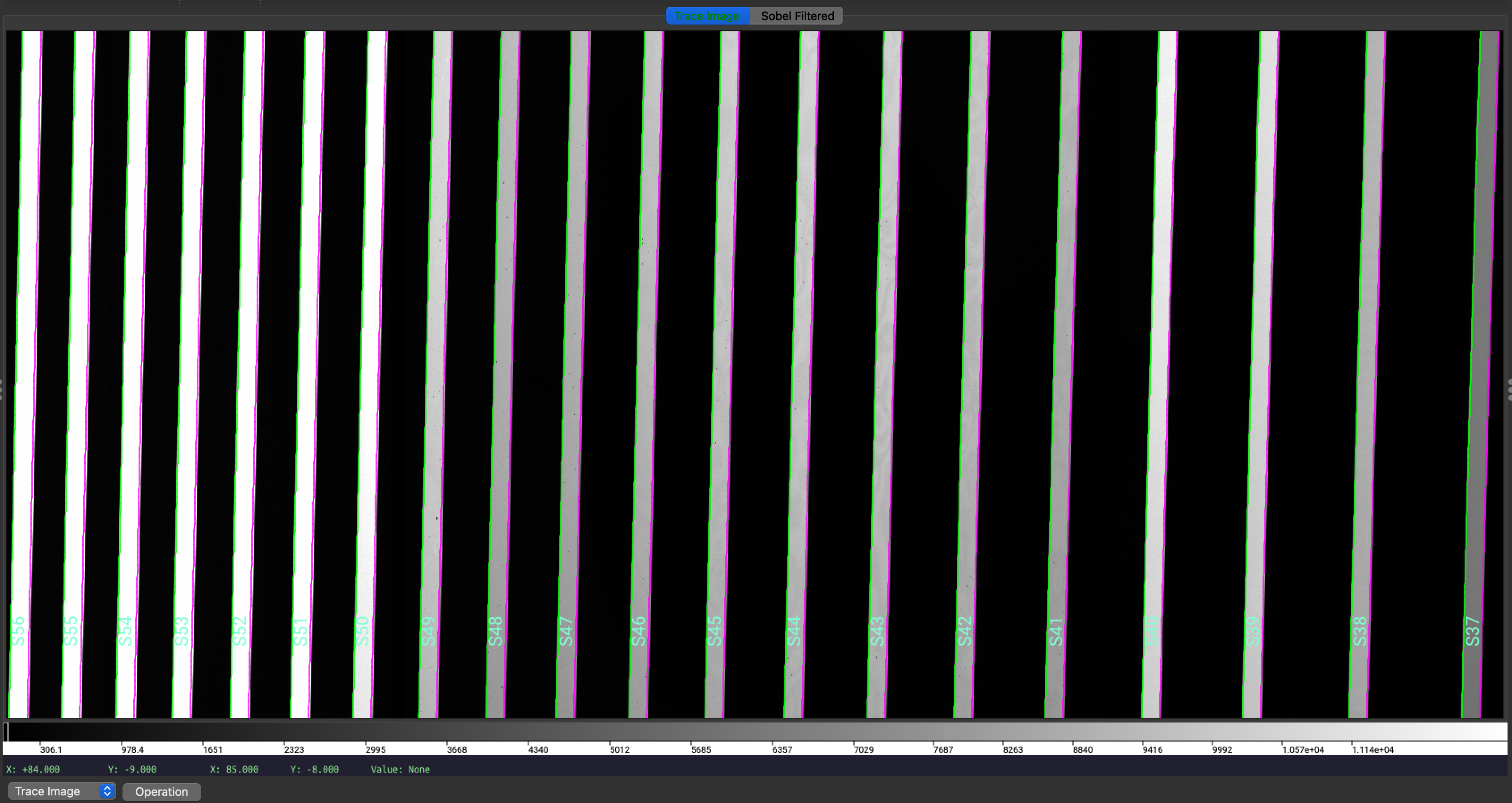
Trace Image, i.e., the flat image, with the traced order edges overlaid.
The green/magenta lines indicate the left/right order edges, and the aquamarine
labels starting with an S are the internal slit/order identifiers of PypeIt.
Additionally, since for echelle observations PypeIt is able to add missing orders, a QA
file is automatically generated to allow the user to assess the success of the predicted locations;
see Echelle Order Prediction.
The QA file is a PNG file in the QA/PNG/ folder and it looks like this:
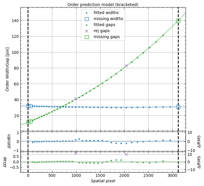
QA plot, called Edges_A_0_MSC01_orders_qa.png, showing the measured order
spatial widths (blue) and gaps (green) in pixels. The colored lines show
the best fit polynomial model used for the predicted order locations. The
missing orders that are added are shown as open squares.
Wavelengths
The wavelength calibration is usually performed using the ThAr arc lamp frames, and an approach that is specific for Echelle Spectrographs. This approach follows the standard procedure for the 1D wavelength fit, but it also performs a 2D fit to the wavelength solutions in order to improve the 1D fits. The 2D fit is performed on a per detector basis, since we find the solution for the whole mosaic to be less accurate.
Below is the 1D fit wavelength-calibration QA plot for the bluest order in this dataset (order=62). Such a plot is produced for each order.
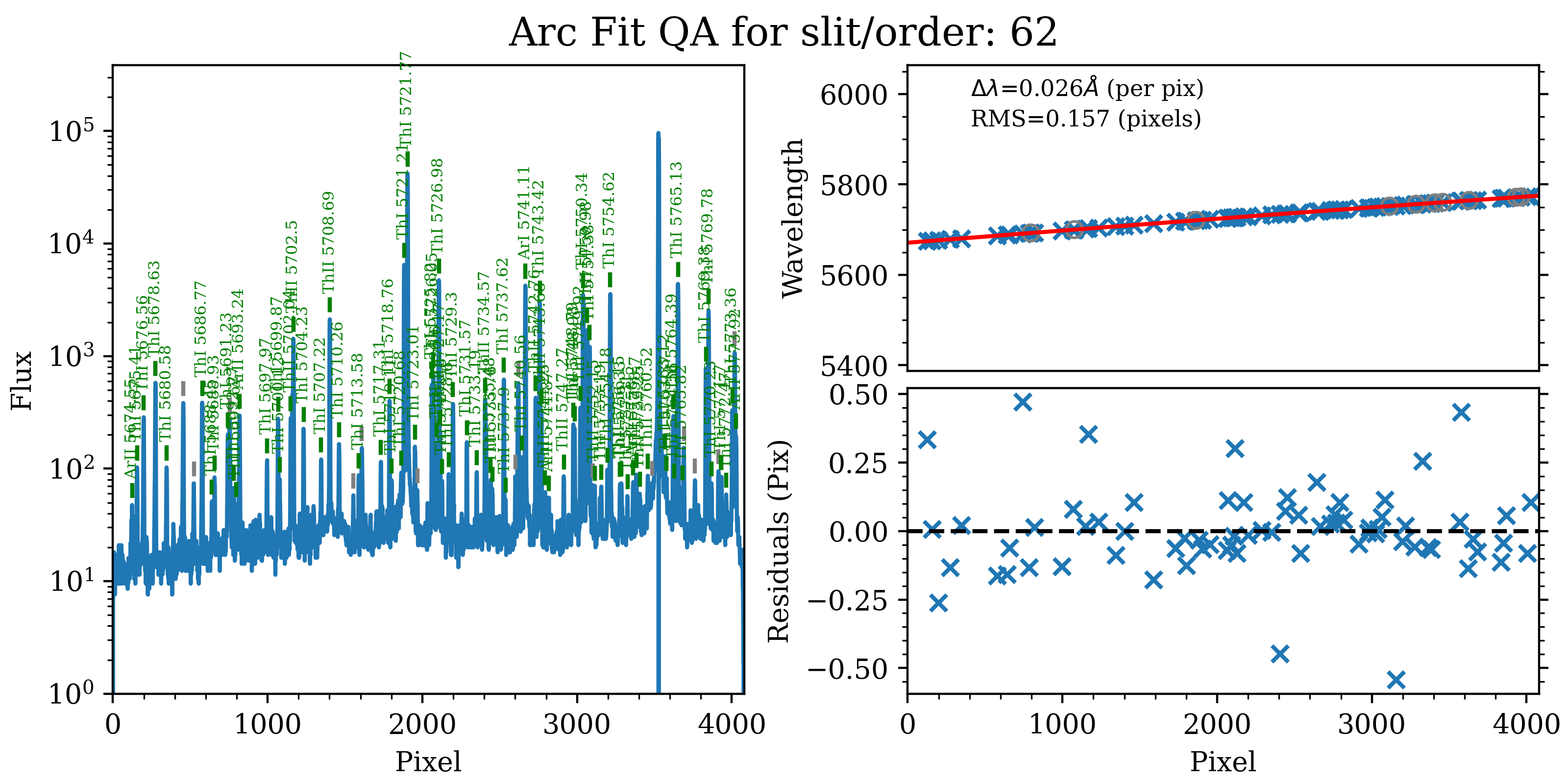
The 1D fit wavelength-calibration QA plot for the bluest Keck/HIRES order
(order=62), called Arc_1dfit_A_0_MSC01_S0062.png. The left panel shows
the arc spectrum extracted down the center of the order, with green text and
lines marking lines used by the wavelength calibration. Gray lines mark
detected features that were not included in the wavelength solution. The
top-right panel shows the fit (red) to the observed trend in wavelength as a
function of spectral pixel (blue crosses); gray circles are features that
were rejected by the wavelength solution. The bottom-right panel shows the
fit residuals (i.e., data - model).
The results of the 2D fit can be inspected by looking at the automatically generated QA files. Below is an example of the global 2D fit and the improved 1D fits QA plots.
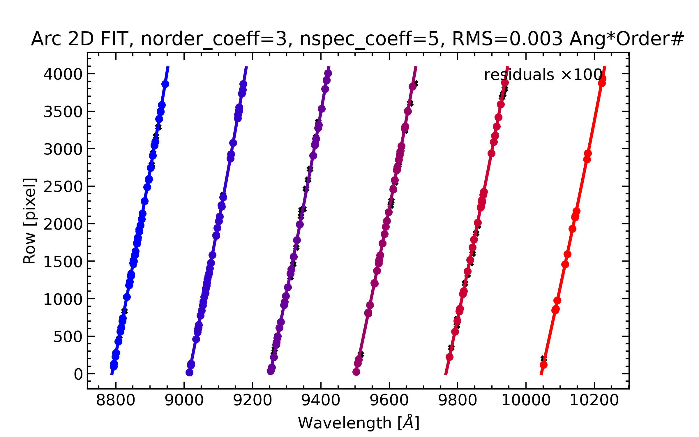
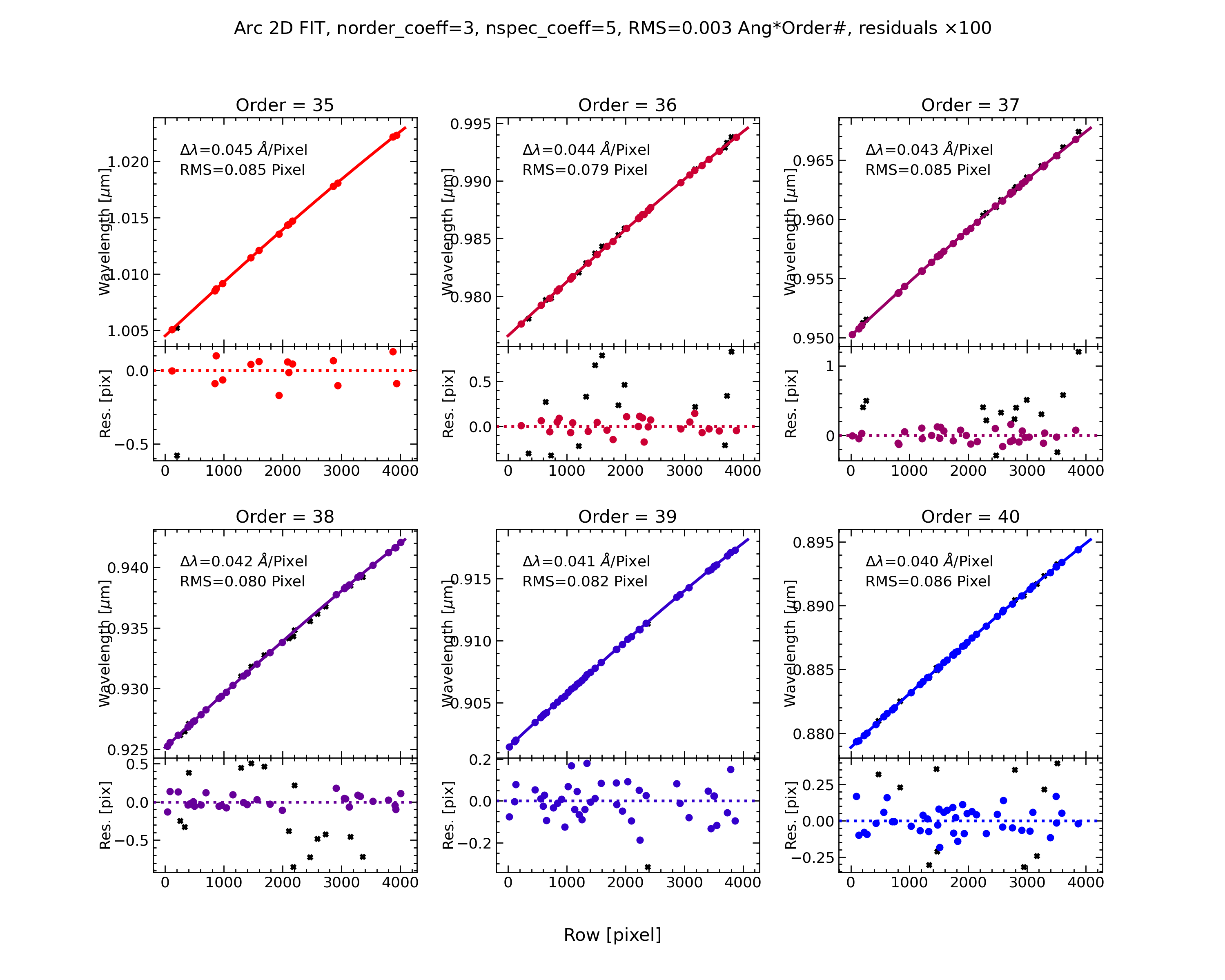
Wavelength-calibration QA plots, showing the global 2D fit (on the left) and the improved 1D fits (on the right) for the six reddest orders in the Keck/HIRES dataset, i.e. the orders in the red ccd.
In addition, the script pypeit_chk_wavecalib provides a summary of the wavelength calibration for all orders. We can run it with this simple call:
pypeit_chk_wavecalib Calibrations/WaveCalib_A_0_MSC01.fits
and it prints on screen the following (here truncated) table:
 N. SpatOrderID minWave Wave_cen maxWave dWave Nlin     IDs_Wave_range    IDs_Wave_cov(%) measured_fwhm  RMS
--- ----------- ------- -------- ------- ----- ---- --------------------- --------------- ------------- -----
  0          62  5671.2   5725.3  5775.1 0.026   72  5674.551 -  5773.924            95.6           4.6 0.157
  1          61  5764.1   5819.1  5869.8 0.026   74  5764.392 -  5868.438            98.4           4.7 0.174
  2          60  5860.1   5916.1  5967.7 0.027   87  5861.293 -  5965.578            96.9           4.7 0.179
  3          59  5959.3   6016.4  6068.9 0.027   73  5961.325 -  6067.459            96.8           4.6 0.097
  4          58  6062.0   6120.1  6173.6 0.028   70  6063.214 -  6171.881            97.3           4.6 0.105
  5          57  6168.3   6227.5  6282.0 0.028   78  6171.529 -  6280.903            96.2           4.7 0.147
See pypeit_chk_wavecalib for a detailed description of all the columns.
Tilts
Wavelength tilts are measured performing a 2D fit to the traced arc lines.
There are several QA files written to the QA/PNG/ folder that can be inspected
to check the quality of the 2D fits. See QA PNG files for examples of these QAs.
The 2D fit for the wavelength tilts can also be inspected using the script pypeit_chk_tilts, which shows a Tiltimg image in a ginga or matplotlib window with the traced and 2D fitted tilts over-plotted. Here is an example:
pypeit_chk_tilts Calibrations/Tilts_A_0_MSC01.fits
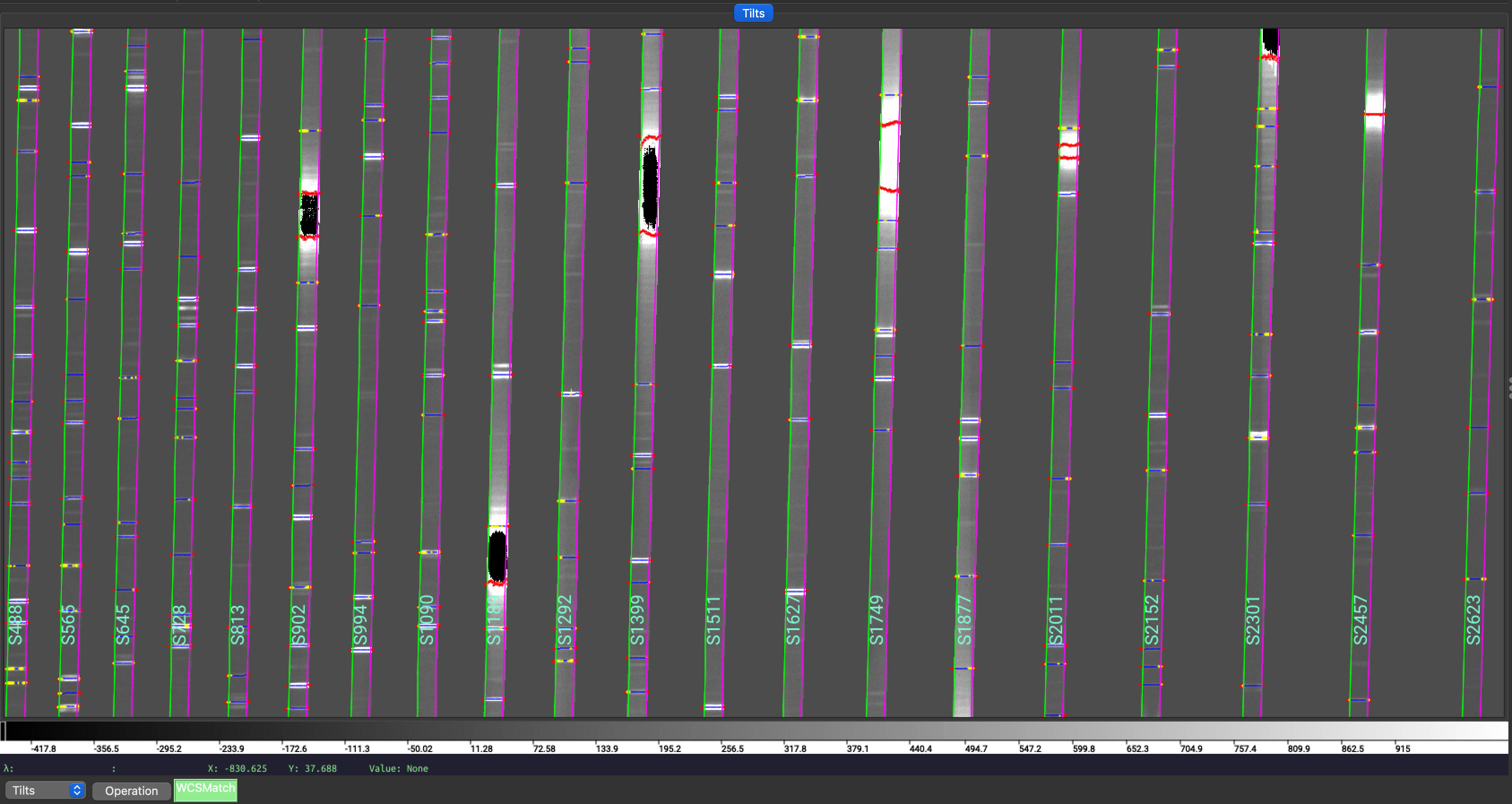
Zoom-in of a Tiltimg image in a ginga window with overlaid the 2D fitted tilts (blue), the masked pixels (red), and the pixels rejected in the 2D fitting (yellow). The lines that are not overlaid with any colored tilts are the ones that were not detected for the purpose of the performing the 2D fitting.
See Tilts for further details.
Flatfield
PypeIt computes a number of multiplicative corrections to correct the 2D spectral response
for pixel-to-pixel detector throughput variations and lower-order spatial and spectral illumination
and throughput corrections. We collectively refer to these as flat-field corrections; see
here and here.
To inspect the Flat images we can use the script pypeit_chk_flats, with this explicit call:
pypeit_chk_flats Calibrations/Flat_A_0_MSC01.fits
This script displays a series of flat fielding images in a ginga viewer, each in a separate tab. See Flat and Flat Fielding for further details.
Object Finding and Extraction
After the above calibrations are complete, PypeIt will iteratively identify sources, perform global and local sky subtraction, and perform 1D spectral extractions. This process is fully described here: Object Finding.
PypeIt produces QA files that allow you to assess the detection of the objects. For example, here is the QA plots for the quasar and standard star spectra in order 35 (reddest order):
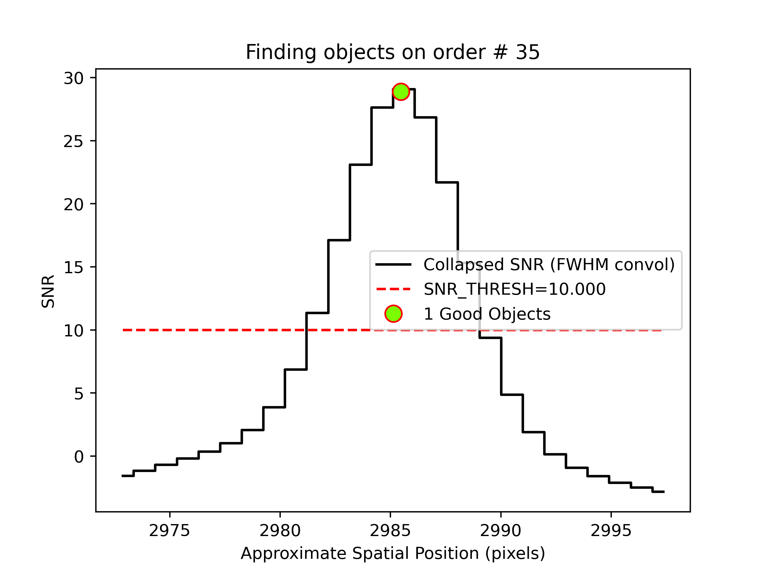
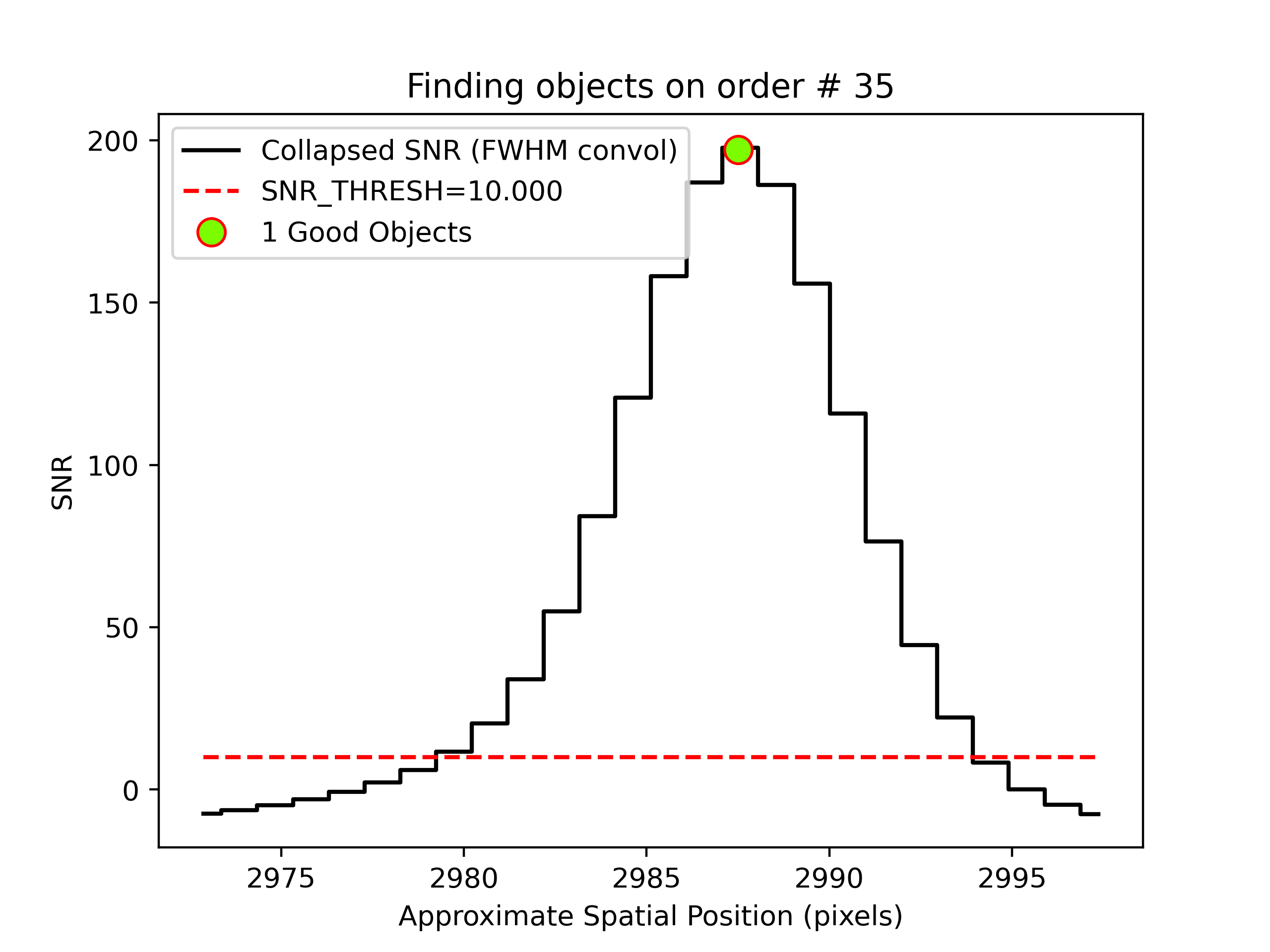
Detection of the quasar (left) and standard star (right) in order 35 spectra.
The black line shows the spectrally collapsed S/N as a function of position within the order.
The dashed red line is the S/N threshold set by the FindObjPar Keywords,
and the green circle marks the spatial position of the detected object. This plot
is useful to assess if the object was correctly detected and if the S/N threshold
(snr_thresh) parameter set is appropriate for the observation.
Given that HIRES produces multi-order echelle data, PypeIt will attempt to extract the object spectrum across all orders, even if it is only detected in a single order. Therefore, PypeIt uses the provided standard spectrum as a crutch to trace the relative spatial position of the object spectrum in all orders.
Outputs
The primary science output from run_pypeit are 2D spectral images and 1D
spectral extractions, located in the Science/ folder.; see Spec2D Output
and Spec1D Output.
Spec2D
The calibrated 2D spectral images can be visually inspected using pypeit_show_2dspec, which displays the images in a ginga window. The call to visualize the 2D spectral image of one of the quasar observations is:
pypeit_show_2dspec Science/spec2d_HI.20151214.17593-SDSSJ0100+2802_HIRES_20151214T045314.323.fits
We show here a zoom-in screenshot from three (sciimg-DET01, sky_resid-DET01, resid-DET01) of the
four tabs in the ginga window:
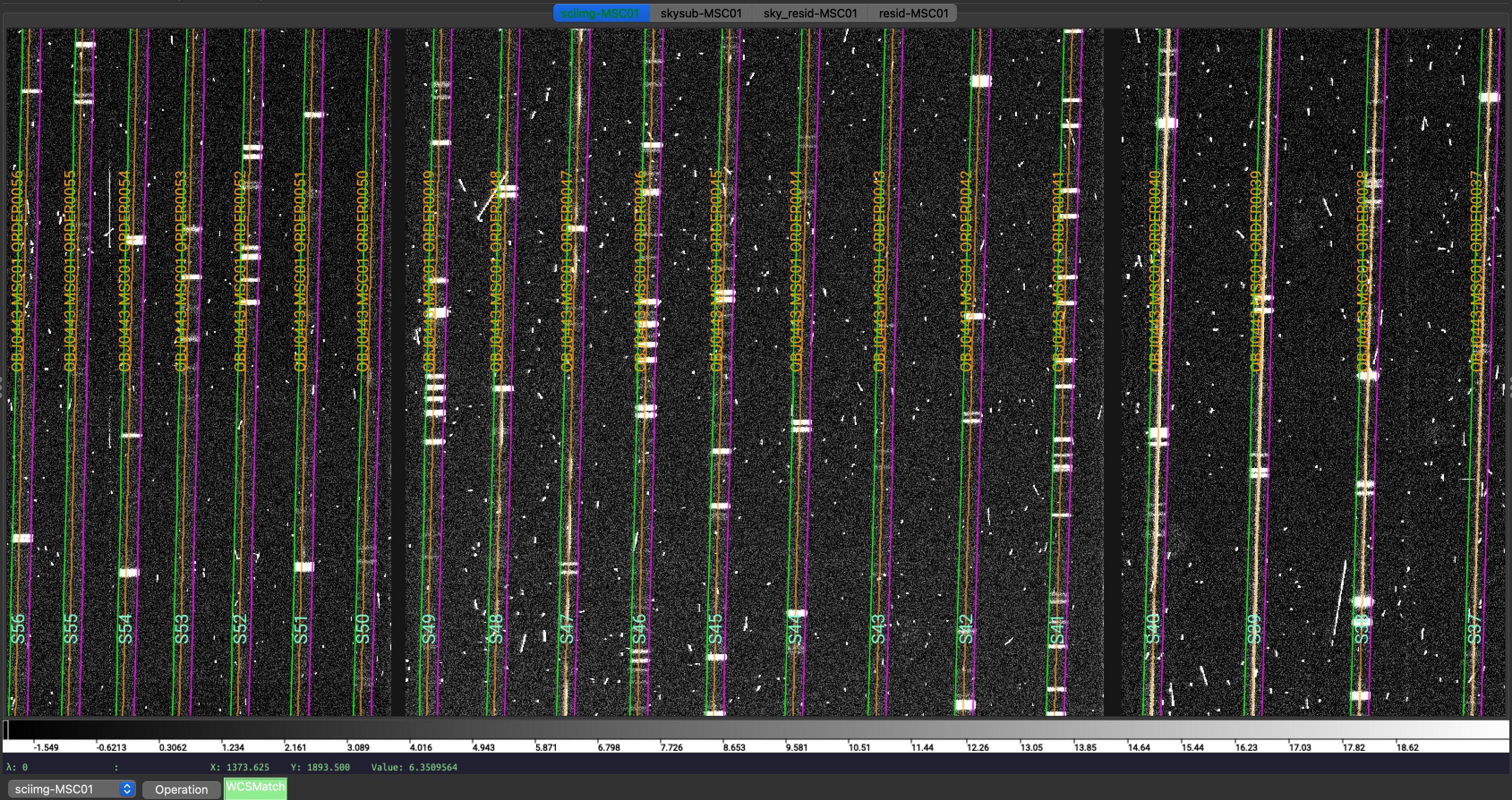
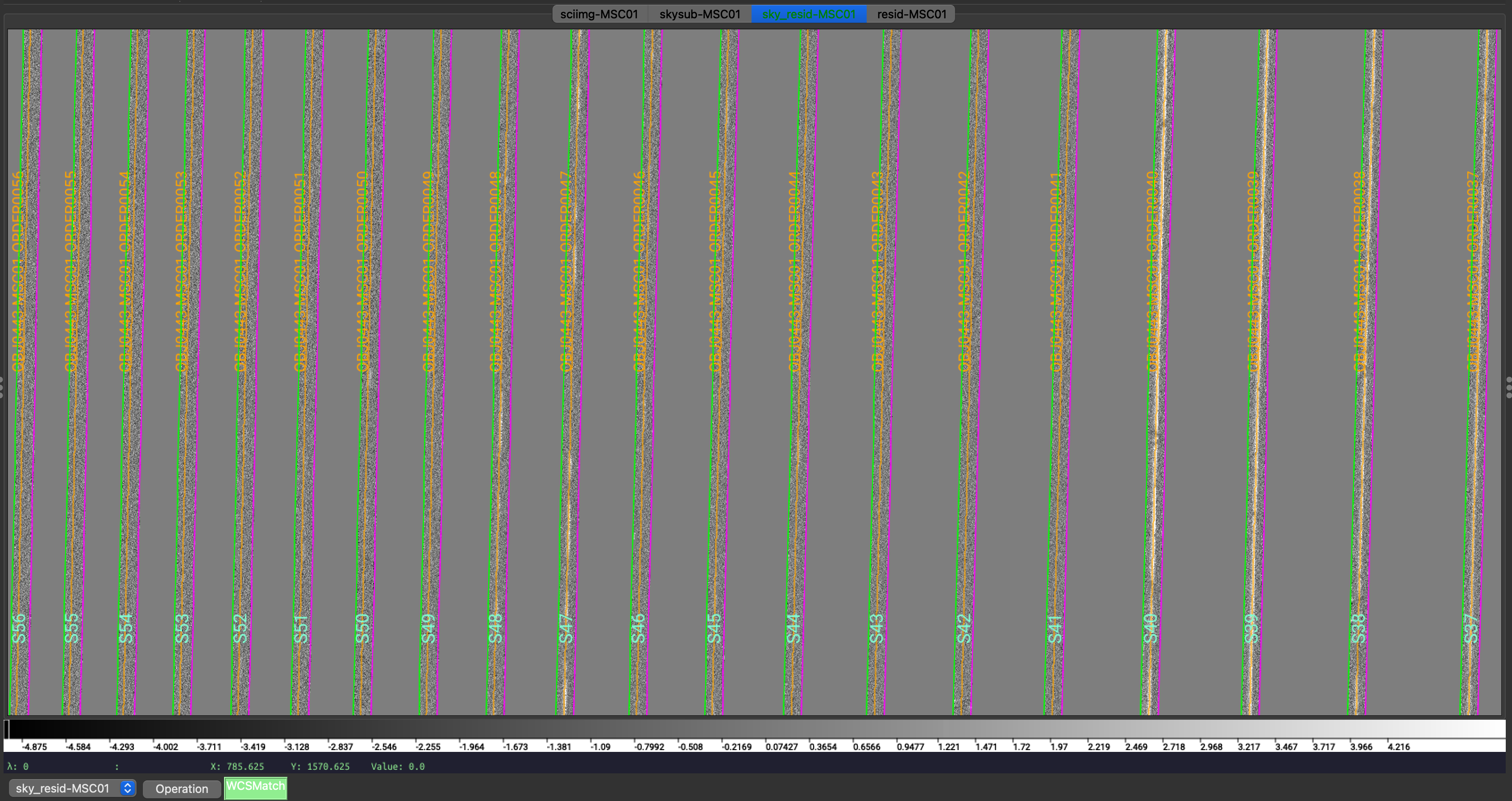
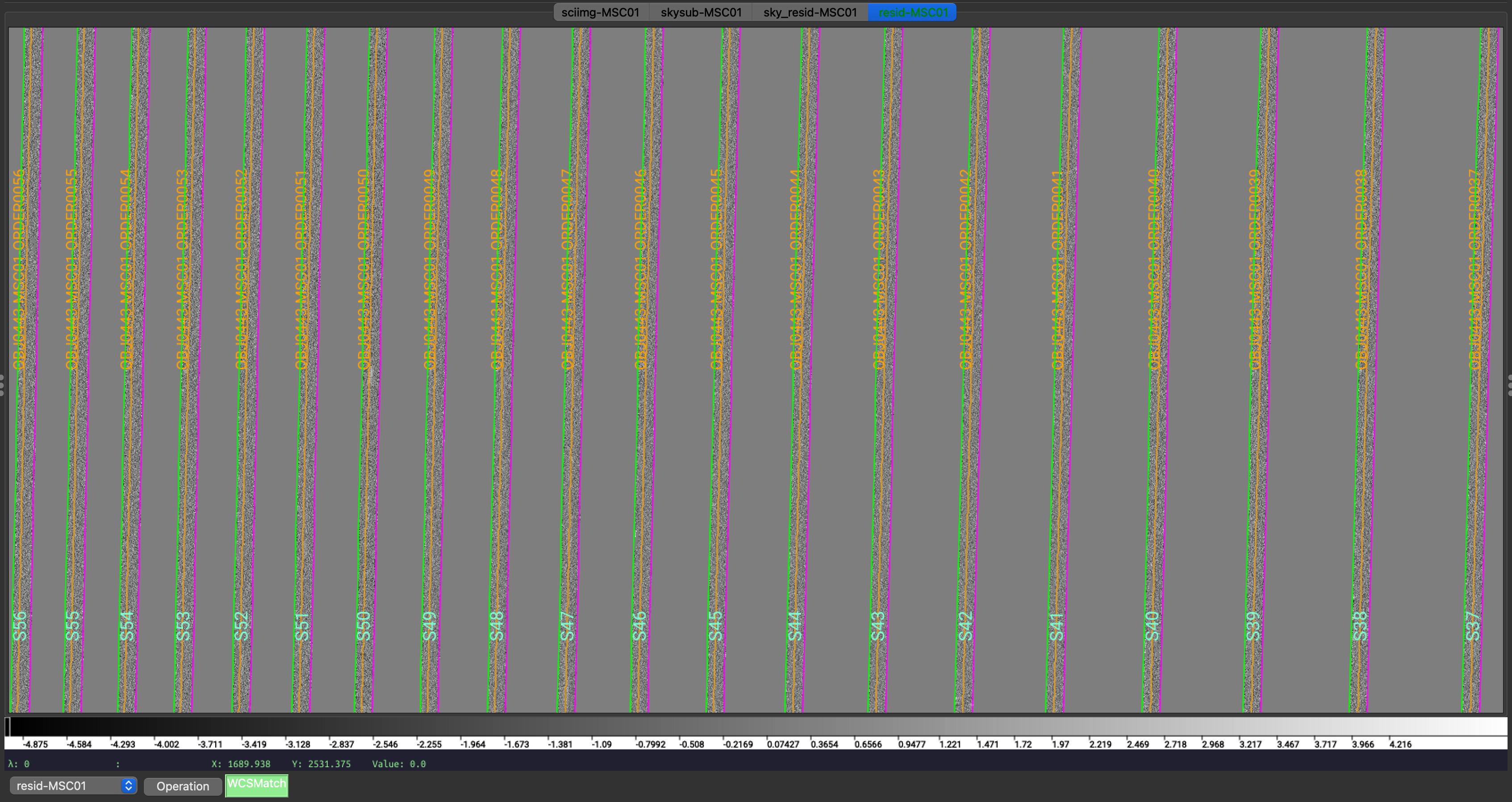
Calibrated science image at the top, in the middle the sky residual image (sky-subtracted
calibrated image divided by the uncertainties), and on the right the residual image.
The green/magenta lines are the order edges. The orange lines are the object traces and the
orange text is the PypeIt assigned name (starting with OBJ ).
The main assessments to perform are to make sure that the object is well traced,
that there are little to no strong sky residuals in the sky_resid channel,
and that the data in the resid channel looks like pure noise (see also pypeit_chk_noise_2dspec).
Spec1D
A summary of all the extracted sources is reported in an ASCII text with the
same name as the spec1d fits file, but with the extension changed from .fits to .txt.
For this example, here are the first few lines of the file
Science/spec1d_HI.20151214.17593-SDSSJ0100+2802_HIRES_20151214T045314.323.txt:
| order |          name | spat_pixpos | spat_fracpos | box_width | opt_fwhm |   s2n | wv_rms |
|    62 | OBJ0443-MSC01 |        66.2 |        0.443 |      3.00 |    0.804 | -0.01 |  0.157 |
|    61 | OBJ0443-MSC01 |       130.6 |        0.443 |      3.00 |    0.804 | -0.02 |  0.174 |
|    60 | OBJ0443-MSC01 |       197.2 |        0.443 |      3.00 |    0.804 | -0.02 |  0.179 |
|    59 | OBJ0443-MSC01 |       265.8 |        0.443 |      3.00 |    0.804 | -0.01 |  0.097 |
|    58 | OBJ0443-MSC01 |       336.5 |        0.443 |      3.00 |    0.804 |  0.01 |  0.105 |
It shows a table with the PypeIt names of the extracted spectra in each order and all the associated information about the extraction. See Extraction Information for a detailed description of this file. Each spectrum is given its own extension in the fits file, where the extension name is based on the object name identified in the file and the order number; e.g., OBJ0443-MSC01-ORDER0040.
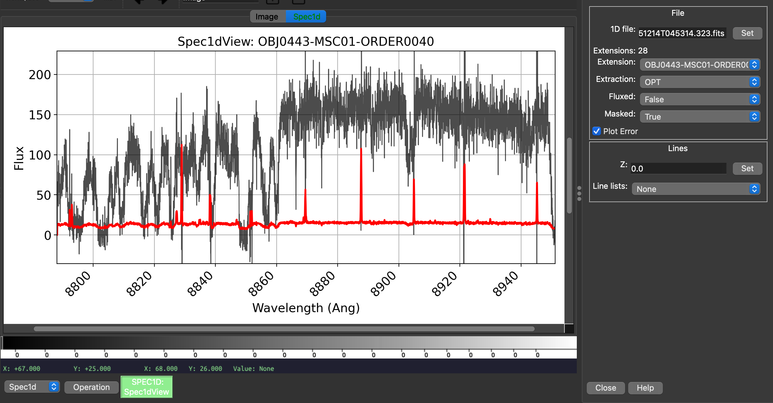
You can plot the spectrum using pypeit_show_1dspec:
pypeit_show_1dspec Science/spec1d_HI.20151214.17593-SDSSJ0100+2802_HIRES_20151214T045314.323.fits
which plots the spectrum in a tab of the ginga viewer and allows you to select the different order spectra using a drop down menu, in addition to selecting other properties of the spectrum. Here is an example:
Fluxing and co-adding
The flux calibration is performed by first creating a sensitivity function from the standard star observations. The sensitivity function is then applied to the science observations. See Fluxing for more details.
Caution
High quality absolute flux calibration of HIRES data is difficult to achieve. This is due to the fact that the instrument’s response function varies with the telescope position in an “unpredictable way”, see Suzuki at al 2003 and here. The following steps, therefore, provide an approximate relative flux calibration. The user should be aware of this and use the flux calibration with caution.
Generating a Sensitivity function
The sensitivity function is generated by the pypeit_sensfunc script, using the standard star observations reduced in the Main Run. The typical call for HIRES is:
pypeit_sensfunc -f Science/spec1d_HI.20151214.16715-Feige110_HIRES_20151214T043836.845.fits
The -f flag requests that the script uses the extracted spectrum of the flatfield calibration to
estimate the blaze function in order to improve the sensitivity function calculation. Other parameters
can be set through a configuration file, but in this case, most of the parameters needed for HIRES
are already set by default. See SensFuncPar Keywords for a list of all the parameters that can be set,
and KECK HIRES (keck_hires) for the default parameters for HIRES.
The script produces a sensitivity function file, called
sens_HI.20151214.16715-Feige110_HIRES_20151214T043836.845.fits and three QA files that can be
inspected to assess the quality of the sensitivity function.
One QA file shows the fit, per order, of the sensitivity function zeropoint, another shows the computed throughput
for the current observation, and the last one shows the standard star spectrum flux-calibrated using
the generated sensitivity function. Here is an example of the zeropoint fit QA plot and the flux-calibrated
standard star spectrum:
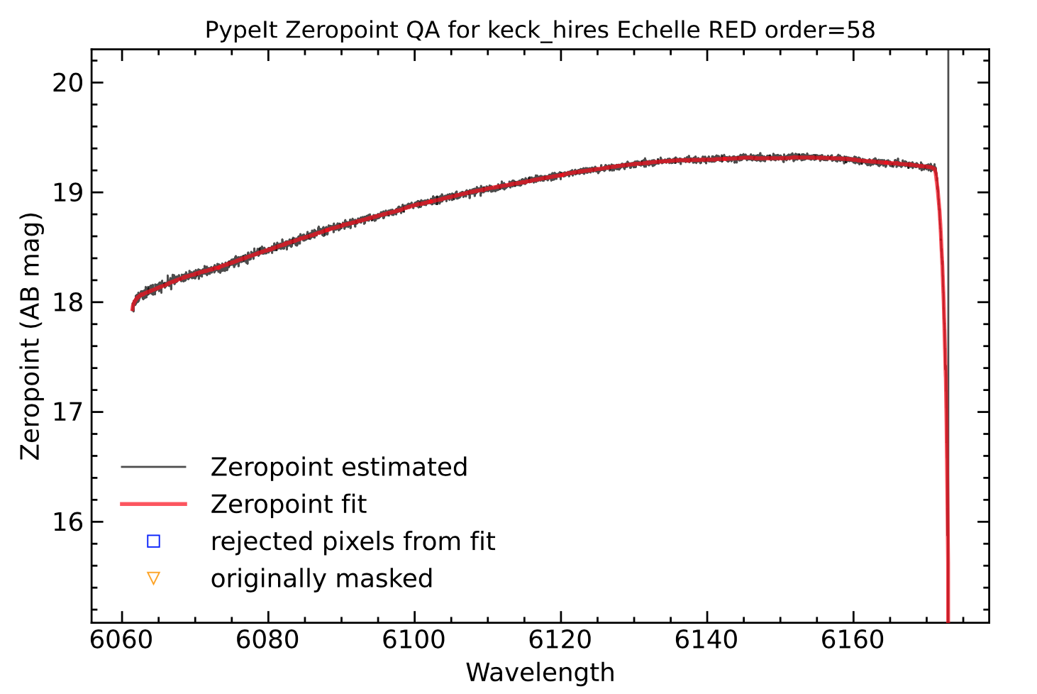
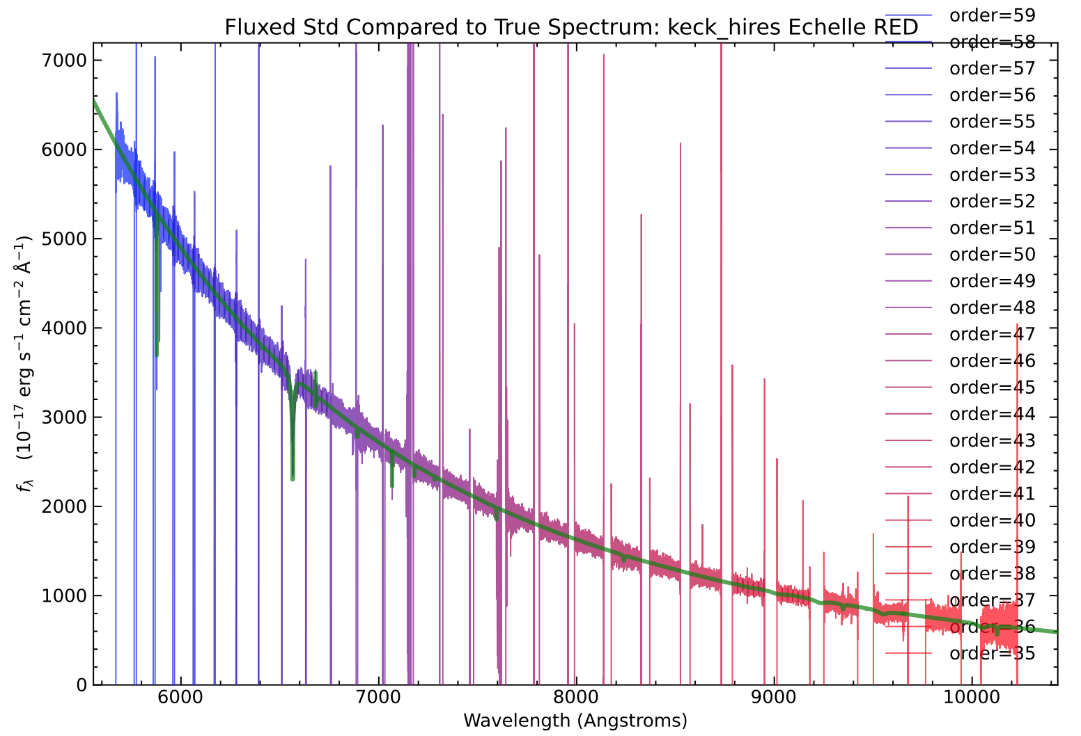
On the left, example of the spectroscopic zeropoint fit for order 58. On the right, the standard star spectrum flux-calibrated using the generated sensitivity function. The true archival standard star spectrum is also shown in green for comparison.
Flux Calibration
For the next steps we need specific configuration files, which can be generated using the pypeit_flux_setup script:
pypeit_flux_setup --objmodel qso Science/ ./
This script takes as input the folder where the spec1d files are stored (Science/) and the folder
where the sensitivity function is stored (./). The --objmodel flag is used to specify the type
of object model to be used for the telluric correction. The script creates three configuration files:
keck_hires.flux, keck_hires.coadd1d, and keck_hires.tell.
The keck_hires.flux (see also Flux File) looks like this:
# Auto-generated Flux input file using PypeIt version: 1.17.1.dev42+gcc6463672
# UTC 2025-03-28T00:05:25.103+00:00

# User-defined execution parameters
[fluxcalib]
  extinct_correct = False  # Set to True if your SENSFUNC derived with the UVIS algorithm
# Please add your SENSFUNC file name below before running pypeit_flux_calib

# Data block
flux read
 path .
 path Science
                                                              filename |                                                       sensfile
spec1d_HI.20151214.20581-SDSSJ0100+2802_HIRES_20151214T054302.726.fits | sens_HI.20151214.16715-Feige110_HIRES_20151214T043836.845.fits
      spec1d_HI.20151214.16715-Feige110_HIRES_20151214T043836.845.fits | sens_HI.20151214.16715-Feige110_HIRES_20151214T043836.845.fits
spec1d_HI.20151214.17593-SDSSJ0100+2802_HIRES_20151214T045314.323.fits | sens_HI.20151214.16715-Feige110_HIRES_20151214T043836.845.fits
flux end
It does not need much editing, besides making sure that the sensfile column has the correct file name.
In this example, both the quasar and standard star spectra are flux calibrated.
The flux calibration can be run with:
pypeit_flux_calib keck_hires.flux
This will add a *_FLAM columns to each of the spec1d files in the Science/ directory.
See Current Data Model for more details.
Co-adding
The next step is to co-add the flux-calibrated spectra. This step is particular important for
echelle observations, since the orders are are also stitched together. The co-addition is performed
using the pypeit_coadd_1dspec script and the configuration file keck_hires.coadd1d.
The configuration file (see also coadd1d File) for co-adding the quasar spectra looks like this:
# Auto-generated Coadd1D input file using PypeIt version: 1.17.1.dev42+gcc6463672
# UTC 2025-03-28T00:05:25.115+00:00

# User-defined execution parameters
[coadd1d]
  coaddfile = J0100+2802_coadded_50kms.fits  # Please set your output file name
  wave_method = velocity  # creates a uniformly space grid in log10(lambda)
  dv= 50.0  # km/s

# Data block
coadd1d read
 path .
 path Science
                                                              filename |        obj_id |                                                       sensfile | setup_id
spec1d_HI.20151214.20581-SDSSJ0100+2802_HIRES_20151214T054302.726.fits | OBJ0450-MSC01 | sens_HI.20151214.16715-Feige110_HIRES_20151214T043836.845.fits |        A
spec1d_HI.20151214.17593-SDSSJ0100+2802_HIRES_20151214T045314.323.fits | OBJ0443-MSC01 |                                                                |
coadd1d end
Before running the co-addition, we need to remove the standard star file from the Data Block,
make sure that the sensfile column has the correct file name, and provide a name for the output coaddfile.
In this example, the output file is called J0100+2802_coadded_50kms.fits. If the sensitivity function
used is the same for all the objects, then it is enough to add the file name of the sensitivity function
only to the first row of the Data Block.
In addition, we decided for this example to use a 50 km/s dispersion for the co-added spectrum,
by setting the parameter dv = 50.0, which allows for a smoother visualization of the final spectrum.
The co-addition can then be run with:
pypeit_coadd_1dspec keck_hires.coadd1d
The coadded spectrum can be visualized by just using matplotlib, or we can take advantage of the specutils interface available through PypeIt. Use of this interface requires to have the specutils package installed.
This interface allows us to interact with our spectrum using jdaviz. Although jdaviz can be run both within a jupyter notebook and as a stand-alone application, in order to be able to visualize PypeIt 1D output files, jdaviz must currently be run from within a jupyter notebook. See specutils Interface for more details.
The following lines can be used to load and visualize the co-added spectrum of the quasar J0100+2802:
from pypeit.specutils import Spectrum
from jdaviz import Specviz

file = 'J0100+2802_coadded_50kms.fits'
spec = Spectrum.read(file)

specviz = Specviz()
specviz.load_data(spec)
specviz.show()
Here is an example of how the spectrum looks in the jdaviz interface:
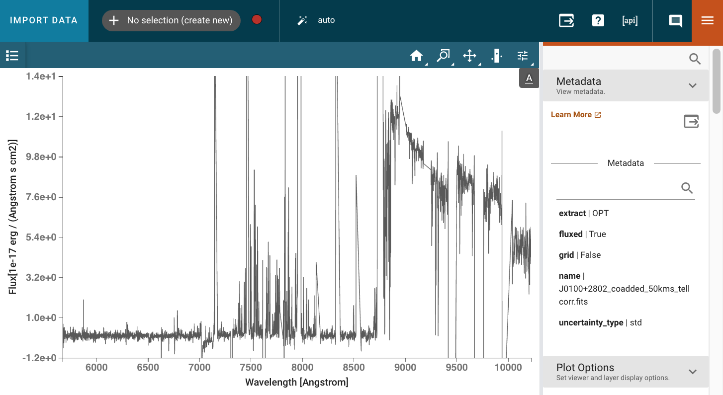
The co-added spectrum of the quasar J0100+2802 at z=6.29, with a 50 km/s dispersion, visualized using the jdaviz interface.
Telluric Correction
Last step that can be performed, if needed, is the telluric correction. This is done using the
pypeit_tellfit script and the configuration file keck_hires.tell. The configuration file
looks like this:
# Auto-generated Telluric input file using PypeIt version: 1.17.1.dev42+gcc6463672
# UTC 2025-03-28T00:05:25.116+00:00

# User-defined execution parameters
[telluric]
  objmodel = qso
  redshift = 6.29
  bal_wv_min_max = 10000., 11000.
The telluric correction relies on a user-defined object model, defined by the objmodel parameter.
In this example, we are using a quasar model, and we needs to edit the configuration file to provide
the redshift of the quasar. The rest of the parameters can be left as default. See TelluricPar Keywords for
a list of all the parameters that can be set, and KECK HIRES (keck_hires) for the default parameters
for HIRES.
The telluric correction can then be run with:
pypeit_tellfit -t keck_hires.tell J0100+2802_coadded_50kms.fits
This will produce a telluric corrected spectrum, with the suffix _tellcorr, which can still be visualized
using the specutils interface as shown above, and a file with the suffix _tellmodel that contains the
telluric model used to correct the spectrum.