Subaru-FOCAS HOWTO
Overview
This doc goes through a full run of PypeIt on one of our Subaru FOCAS
long-slit datasets, specifically the subaru_focas/300R_O58
dataset. These are Subaru/FOCAS long-slit observations taken with the
SCFCGRMR01 grating and SCFCSLLC08 decker. See here
to find the example dataset.
If you’re having trouble reducing your data, we encourage you to try going through this tutorial using this example dataset first. Please join our PypeIt Users Slack using this invitation link to ask for help, and/or Submit an issue to Github if you find a bug!
The following was performed on a Dell laptop with 64 Gb RAM, but we expect 16Gb of RAM would be sufficient for this dataset.
Setup
Organize data
Identify the folder where the raw data are stored and make sure you have
all the calibration files you need, in addition to the science ones.
In this example, the raw data are stored in the folder
/PypeIt-development-suite/RAW_DATA/subaru_focas/300R_O58.
The files within this folder are:
$ ls -1
FCSA00216184.fits
FCSA00216242.fits
FCSA00216518.fits
FCSA00216218.fits
FCSA00216334.fits
This folder can include data from different datasets (e.g., more than one decker or observations with various gratings). The script pypeit_setup (see next step) will help to parse the desired dataset.
Run pypeit_setup
The first script to run with PypeIt is pypeit_setup, which examines the raw files and generates a sorted list and (when instructed) one PypeIt Reduction File per instrument configuration.
See complete instructions provided in Setup.
For this example, we move to the folder where we want to perform the reduction and save the associated outputs and we run:
cd folder_for_reducing
pypeit_setup -s subaru_focas -r ../../../RAW_DATA/subaru_focas/300R_O58/FCSA00216 -G
This launches the pypeit_setup GUI, which allows us to select the dataset we want to reduce. Here is a screenshot of the “A” tab:
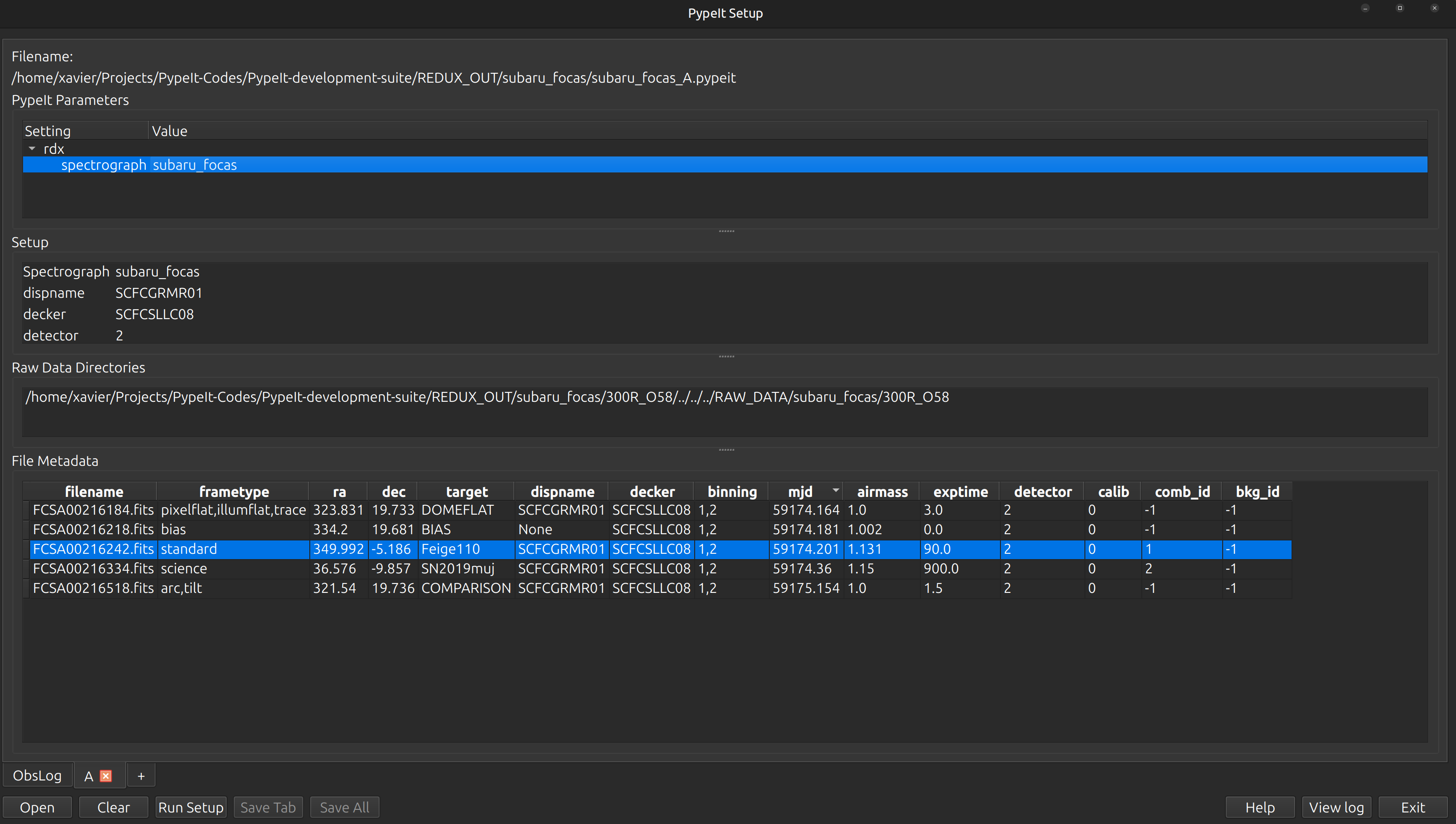
In this case, all of the files have already been selected
to have a similar setup (i.e., same grating, decker, binning, etc.).
But one of the files (FCSA00216242.fits) is mis-typed as a science
frame instead of a standard star. We change the frametype of this
file to standard and then click on the Save All button.
This writes the PypeIt Reduction File called subaru_focas_A.pypeit:
# User-defined execution parameters
[rdx]
    spectrograph = subaru_focas
[reduce]
    [[findobj]]
        maxnumber_sci = 2

# Setup
setup read
Setup A:
decker: SCFCSLLC08
detector: '2'
dispname: SCFCGRMR01
setup end

# Data block
data read
path /home/xavier/Projects/PypeIt-Codes/PypeIt-development-suite/REDUX_OUT/subaru_focas/300R_O58/../../../RAW_DATA/subaru_focas/300R_O58
        filename |                 frametype |                ra |                dec |     target |   dispname |     decker | binning |            mjd | airmass | exptime | detector | calib | comb_id | bkg_id
FCSA00216518.fits |                  arc,tilt |       321.5400125 | 19.736150000000002 | COMPARISON | SCFCGRMR01 | SCFCSLLC08 |     1,2 | 59175.15442112 |     1.0 |     1.5 |        2 |     0 |      -1 |     -1
FCSA00216218.fits |                      bias | 334.1996666666666 |  19.68111111111111 |       BIAS |       None | SCFCSLLC08 |     1,2 | 59174.18107209 |   1.002 |     0.0 |        2 |     0 |      -1 |     -1
FCSA00216184.fits | pixelflat,illumflat,trace |       323.8308125 |  19.73326111111111 |   DOMEFLAT | SCFCGRMR01 | SCFCSLLC08 |     1,2 | 59174.16350372 |     1.0 |     3.0 |        2 |     0 |      -1 |     -1
FCSA00216242.fits |                   standard | 349.9921499999999 |            -5.1864 |   Feige110 | SCFCGRMR01 | SCFCSLLC08 |     1,2 | 59174.20096207 |   1.131 |    90.0 |        2 |     0 |       1 |     -1
FCSA00216334.fits |                   science | 36.57612916666667 | -9.856508333333332 |  SN2019muj | SCFCGRMR01 | SCFCSLLC08 |     1,2 | 59174.36002913 |    1.15 |   900.0 |        2 |     0 |       2 |     -1
data end
Inspecting this file, we want to make sure that all the frame types were accurately assigned in the
Data Block. If not, these can be fixed by editing the PypeIt Reduction File directly; see instructions
here. We can also remove any bad (or undesired) calibration
or science frames from the list, by either deleting them altogether or commenting them out with a #.
In this case, we have restricted the reduction to
find only 2 objects in the science frames.
This is done by setting the parameter maxnumber_sci to 2
under [reduce][[findobj]] in the PypeIt Reduction File.
Note
PypeIt has a long list of parameters that can be set by the user to customize the reduction. This
makes PypeIt very flexible and able to reduce a wide range of data from many instruments. Most
parameters are set by default for the specific instrument, see SUBARU FOCAS (subaru_focas).
Moreover, there are some parameters that are set by default for a specific configuration within
the same instrument. For example, in many cases, PypeIt uses by default different wavelength templates
for different gratings. The default parameters are not shown in the
PypeIt Reduction File, therefore it may be sometime difficult to know which parameters to set
and which ones to leave as default.
To help with this, the user can inspect the .par file, which is generated at the very beginning
of the main run (see below). This file contains every single available parameter with the assigned
value, giving the user an idea of what are the values of the default parameters.
Main Run
Once the PypeIt Reduction File is ready, the main call is simply:
run_pypeit subaru_focas_A.pypeit -o
The -o flag indicates that any existing output files should be overwritten. As
there are none, it is superfluous but we recommend (almost) always using it.
The code will run uninterrupted until the basic data-reduction procedures (wavelength calibration, field flattening, object finding, sky subtraction, and spectral extraction) are complete; see PypeIt’s Core Data Reduction Executable and Workflow.
As the code processes the data, it will produce a number of files and QA plots that can be inspected. A number of Inspection Scripts are available to help with this process. We present some of these below.
Calibrations
Slit Edges
The code first uses the trace frames to find the slit edges on the detector.
When available, the slitmask design information is used to help find the slit edges
(not for long-slit observations).
To check that PypeIt correctly identified every slits, we can run the pypeit_chk_edges script, with this explicit call:
pypeit_chk_edges Calibrations/Edges_A_0_DET01.fits.gz
which opens the ginga image viewer. Here is a zoom-in screenshot from the first tab in the ginga window:
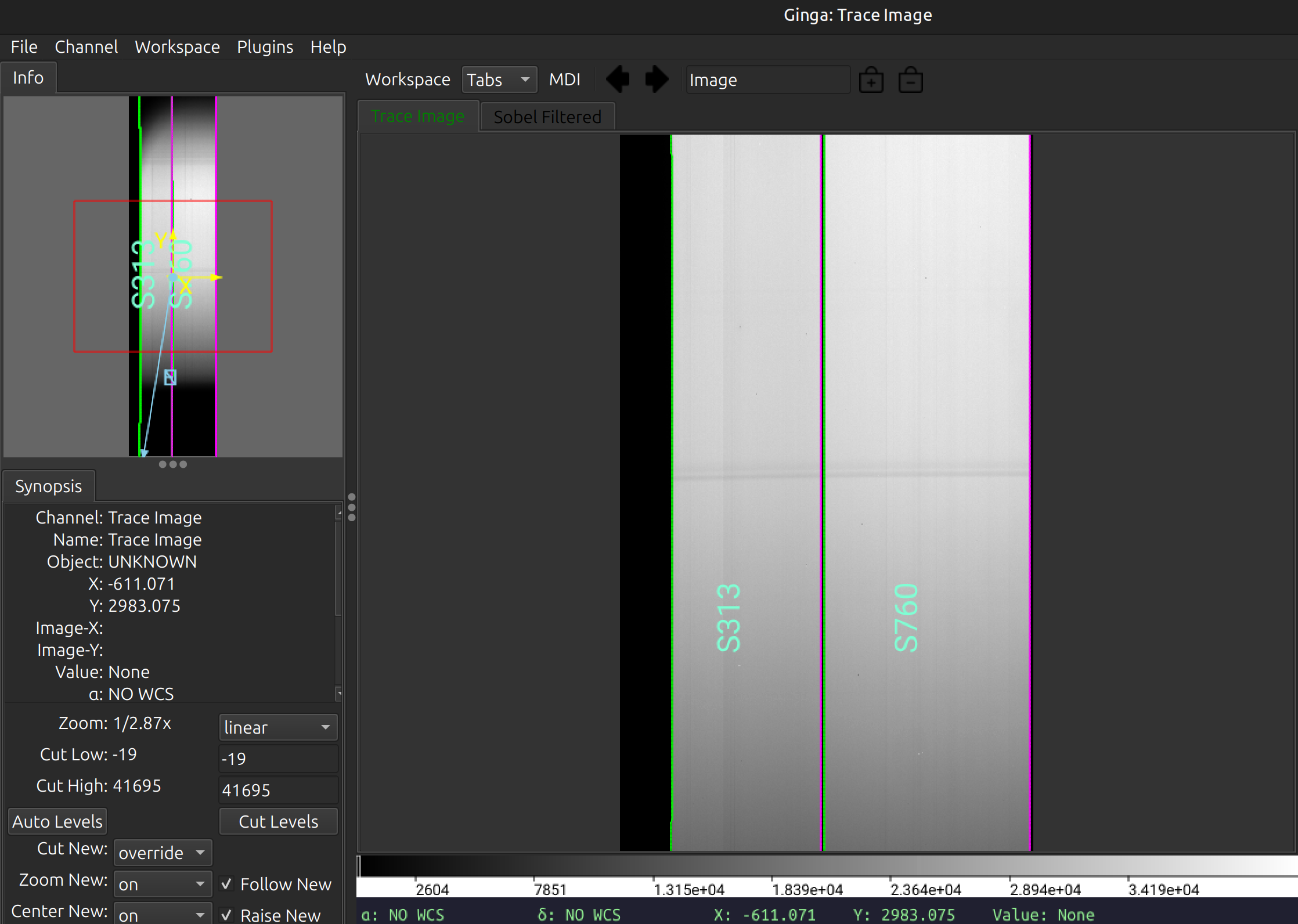
The data shown is the Trace Image, i.e., the flat image.
The green/magenta lines indicate the left/right slit edges.
The aquamarine labels starting with an
S are the internal slit identifiers of PypeIt.
In this case, the code has identified 2 slits on the detector, which is correct.
See Edges for further details.
Arc
You can view the Arc image used for the wavelength calibration of the science frame with ginga:
ginga Calibrations/Arc_A_0_DET01.fits
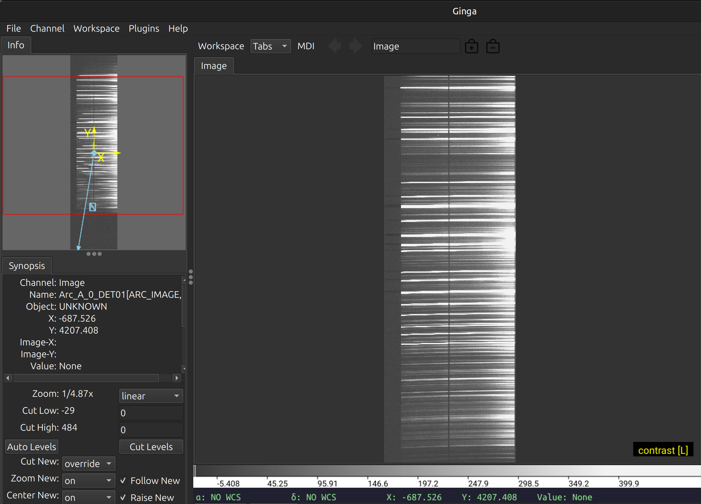
As typical of most arc images, we can see a series of arc lines, here oriented approximately horizontally. It is important to inspect the arc image to make sure it looks good, ensuring to get a good wavelength calibration.
See Arc for further details.
Wavelengths
It is, also, very important to inspect the PypeIt QA for the wavelength calibration.
These are PNG files in the QA/PNG/ folder.
1D
Here is an example of the 1D fits for one of the slit on the detector,
written to the QA/PNGs/Arc_1dfit_A_0_DET01_S0760.png file:
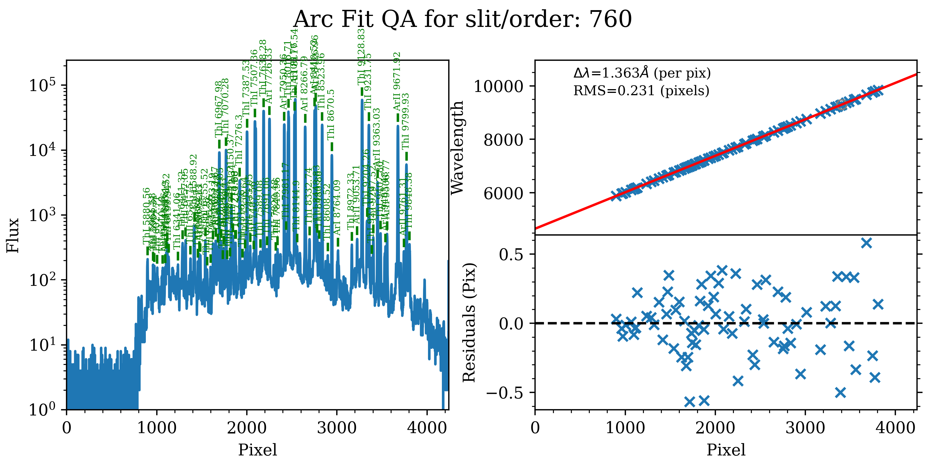
The left panel shows the arc spectrum extracted down the center of the slit, with the lines used by the wavelength calibration marked in green. Gray lines mark detected features that were not included in the wavelength solution. The top-right panel shows the fit (red) to the observed trend in wavelength as a function of spectral pixel (blue crosses); gray circles are features that were rejected by the wavelength solution. The bottom-right panel shows the fit residuals (i.e., data - model).
What you hope to see in this QA is:
On the left, many of the arc lines marked with green IDs
In the upper right, an RMS < 0.3 pixels [depending on binning]
In the lower right, a random scatter about 0 residuals
In addition, the script pypeit_chk_wavecalib provides a summary of the wavelength calibration for all the spectra. We can run it with this simple call:
pypeit_chk_wavecalib Calibrations/WaveCalib_A_0_DET01.fits
and it prints on screen the following table:
N. SpatOrderID minWave Wave_cen maxWave dWave Nlin     IDs_Wave_range    IDs_Wave_cov(%) measured_fwhm  RMS
--- ----------- ------- -------- ------- ----- ---- --------------------- --------------- ------------- -----
0         313  4673.0   7557.1 10434.8 1.358   76  5879.905 -  9848.383            68.9           7.6 0.231
1         760  4658.4   7548.0 10439.9 1.363   77  5880.556 -  9848.383            68.6           8.2 0.231
See pypeit_chk_wavecalib for a detailed description of all the columns.
Tilts
Wavelength tilts are measured performing a 2D fit to the traced arc lines.
There are several QA files written for the 2D fits. One example is
QA/PNGs/Arc_tilts_2d_A_0_DET01_S0760.png:
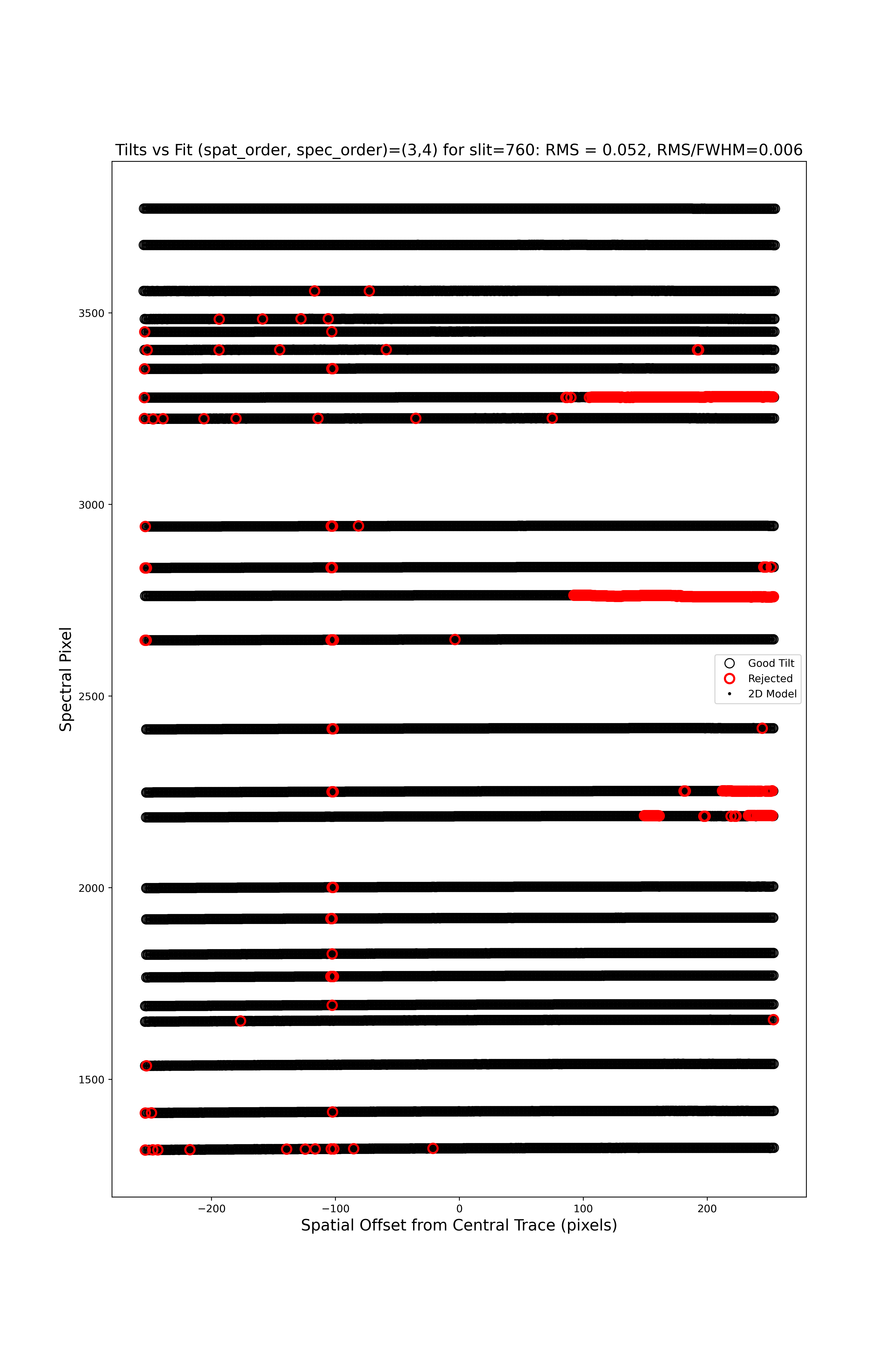
Each horizontal line of black open circles identifies a traced arc line. Red circles shows the points that were rejected in the 2D fitting, and the black points show the model predicted position. The text across the top of the figure gives the RMS of the 2D wavelength solution, which should be less than 0.1 pixels.
The 2D fit for the wavelength tilts can also be inspected using the script pypeit_chk_tilts, which shows a Tiltimg image in a ginga or matplotlib window with the traced and 2D fitted tilts over-plotted.
See Tilts for further details.
Flatfield
PypeIt computes a number of multiplicative corrections to correct the 2D spectral response
for pixel-to-pixel detector throughput variations and lower-order spatial and spectral illumination
and throughput corrections. We collectively refer to these as flat-field corrections; see
here and here.
To inspect the Flat images we can use the script pypeit_chk_flats, with this explicit call:
pypeit_chk_flats Calibrations/Flat_A_0_DET01.fits
Here is a zoom-in screenshot from the first tab in the ginga window (pixflat_norm):
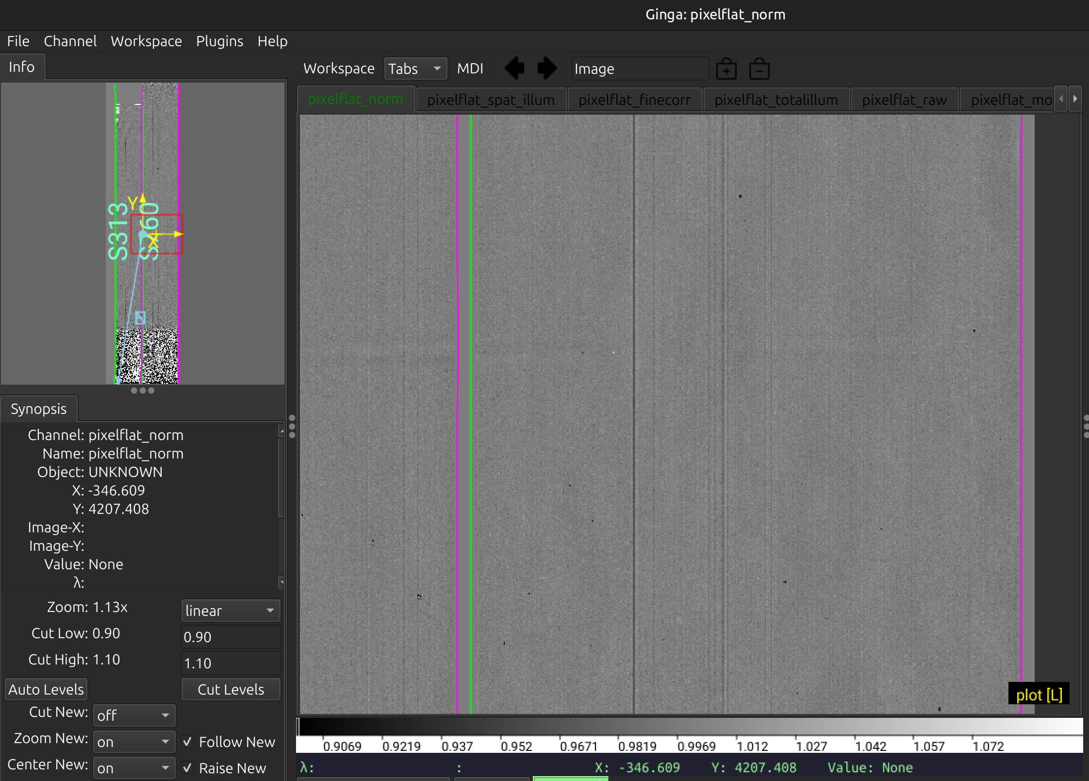
This shows the normalized flat field image. The green/magenta lines are the slit edges, which are tweaked using the illumination flat field.
See Flat and Flat Fielding for further details.
Object finding
After the above calibrations are complete, PypeIt will iteratively identify sources, perform global and local sky subtraction, and perform 1D spectral extractions. This process is fully described here: Object Finding.
PypeIt produces QA files that allow you to assess the detection of the objects.
One example is QA\PNGs\FCSA00216334-SN2019muj_FOCAS_20201121T083826.517_DET01_S0760_obj_prof.png:
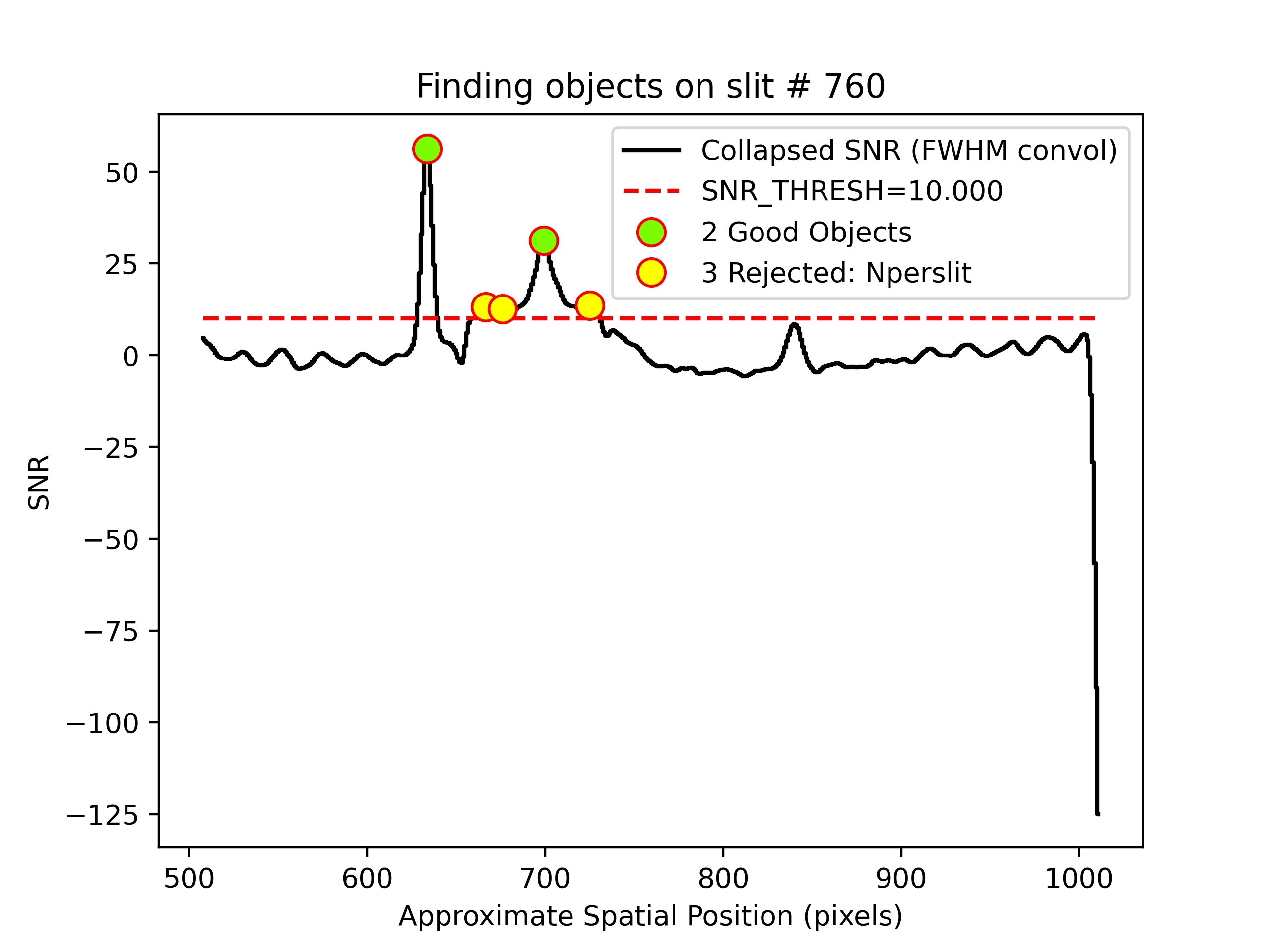
This shows the spatial profile of the object’s S/N collapsed along the spectral direction.
The dashed red line is the S/N threshold set by the FindObjPar Keywords, and the green circle
marks the spatial position of the detected object. This plot is useful to assess if the object
was correctly detected and if the S/N threshold (snr_thresh) set is appropriate for the
observation. You will note that there were 3 objects rejected because we restricted
the code to find only 2 objects in the science frame.
See Object Finding for further details.
Flexure
PypeIt also measures a spectral flexure correction, by performing a cross-correlation
between the sky spectrum extracted in each slit and an archived sky spectrum.
The relative shift between the two spectra is then used to correct the wavelength solution
for each slit (see Spectral Flexure).
Two flexure corrections are computed, one (called global) using the sky lines
extracted at the center of the slit, and one (called local) using the sky lines
extracted at the location of the science object.
There are two QA files (two for the global and two for the local correction)
that can be used to assess the flexure correction. Here is an example of two QA files
for the global correction, called
QA/PNGs/FCSA00216334-SN2019muj_FOCAS_20201121T083826.517_global_DET01_S0760_spec_flex_corr.png
QA/PNGs/FCSA00216334-SN2019muj_FOCAS_20201121T083826.517_global_DET01_S0760_spec_flex_sky.png:
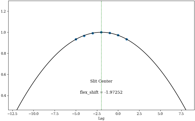
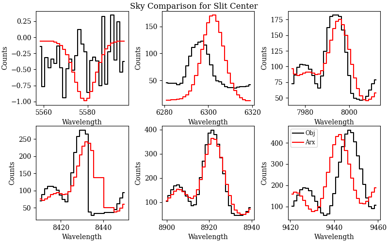
The first plot shows the polynomial fit (black line) between the top seven highest cross-correlation values (y-axis) and the corresponding shift in pixels (x-axis). The value of the shift with the highest cross-correlation is the flexure correction applied to the wavelength solution (also printed in the plot). The user should inspect this plot to make sure that the fit is good and that the value of the flexure shift is comparable to what expected for the observations. The second plot shows sky spectrum cutouts around some of the sky lines used for the flexure correction. The black line is the sky spectrum extracted at the center of the slit shifted by the computed flexure correction, while the red line is the archived sky spectrum. This is another way to assess that the computed flexure correction is good. The user should hope to see a good match between the two spectra.
Outputs
The primary science output from run_pypeit are 2D spectral images and 1D
spectral extractions, located in the Science/ folder.; see Outputs.
Spec2D
Slit inspection
It is frequently useful to view a summary of the slits successfully reduced by PypeIt, by running the script pypeit_parse_slits. In this example, we can inspect the reduced 2D spectrum with this explicit call:
pypeit_parse_slits Science/spec2d_FCSA00216334-SN2019muj_FOCAS_20201121T083826.517.fits
which print the following table in the terminal:
============================== DET01 ==============================
SpatID Flags
------ -----
313  None
760  None
The two columns printed to screen are SpatID (the internal PypeIt ID),
and Flags for each slit.
If the calibration failed for some slits, the Flags column will show the reason for
the failure.
Those slits with None in the Flags column have been successfully reduced.
Visual inspection
The 2D spectrum can be visually inspected using the script pypeit_show_2dspec. In this example, we can visualize the 2D spectrum with this explicit call:
pypeit_show_2dspec Science/spec2d_FCSA00216334-SN2019muj_FOCAS_20201121T083826.517.fits
The --removetrace only shows the object trace in the first channel (the channel showing the
calibrated science image), but does not include it in the remaining channels. It is helpful to
use the --removetrace option to better visualize the object traces (especially for faint
objects).
We show here a zoom-in screenshot from three (sciimg-DET01, skysub-DET01, sky_resid-DET01) of the
four tabs in the ginga window:
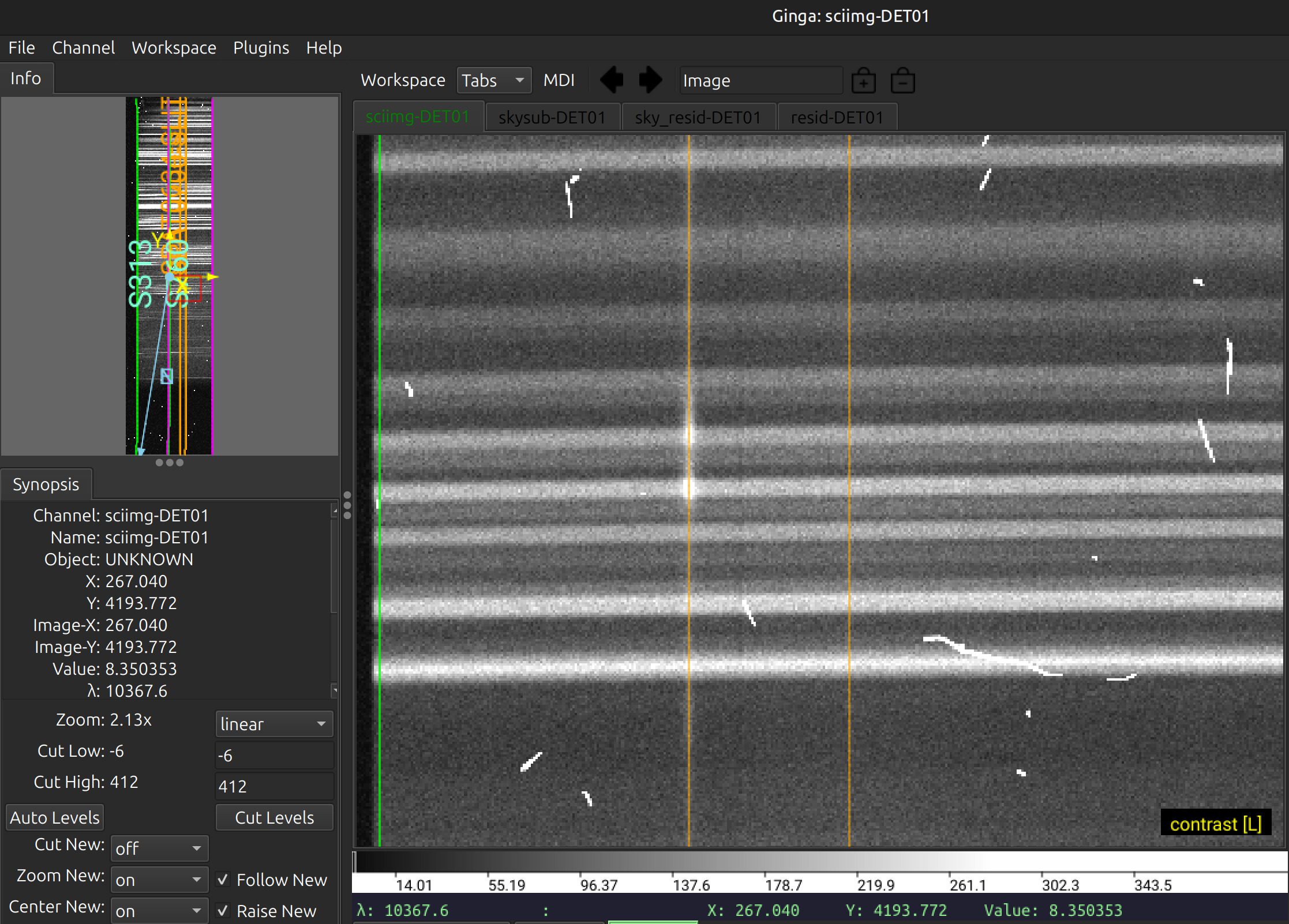
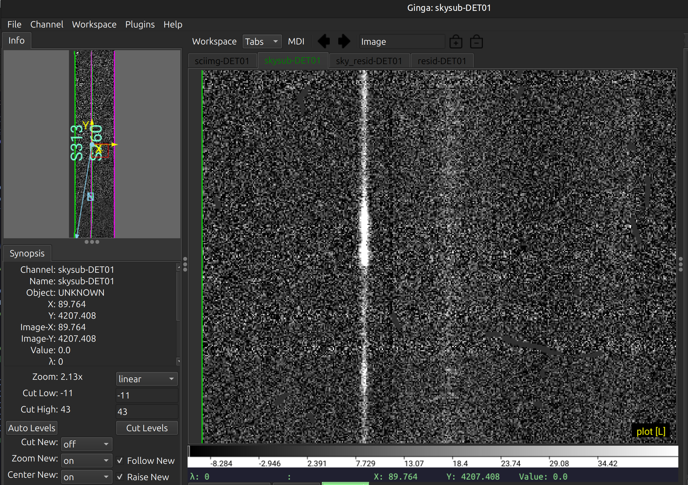
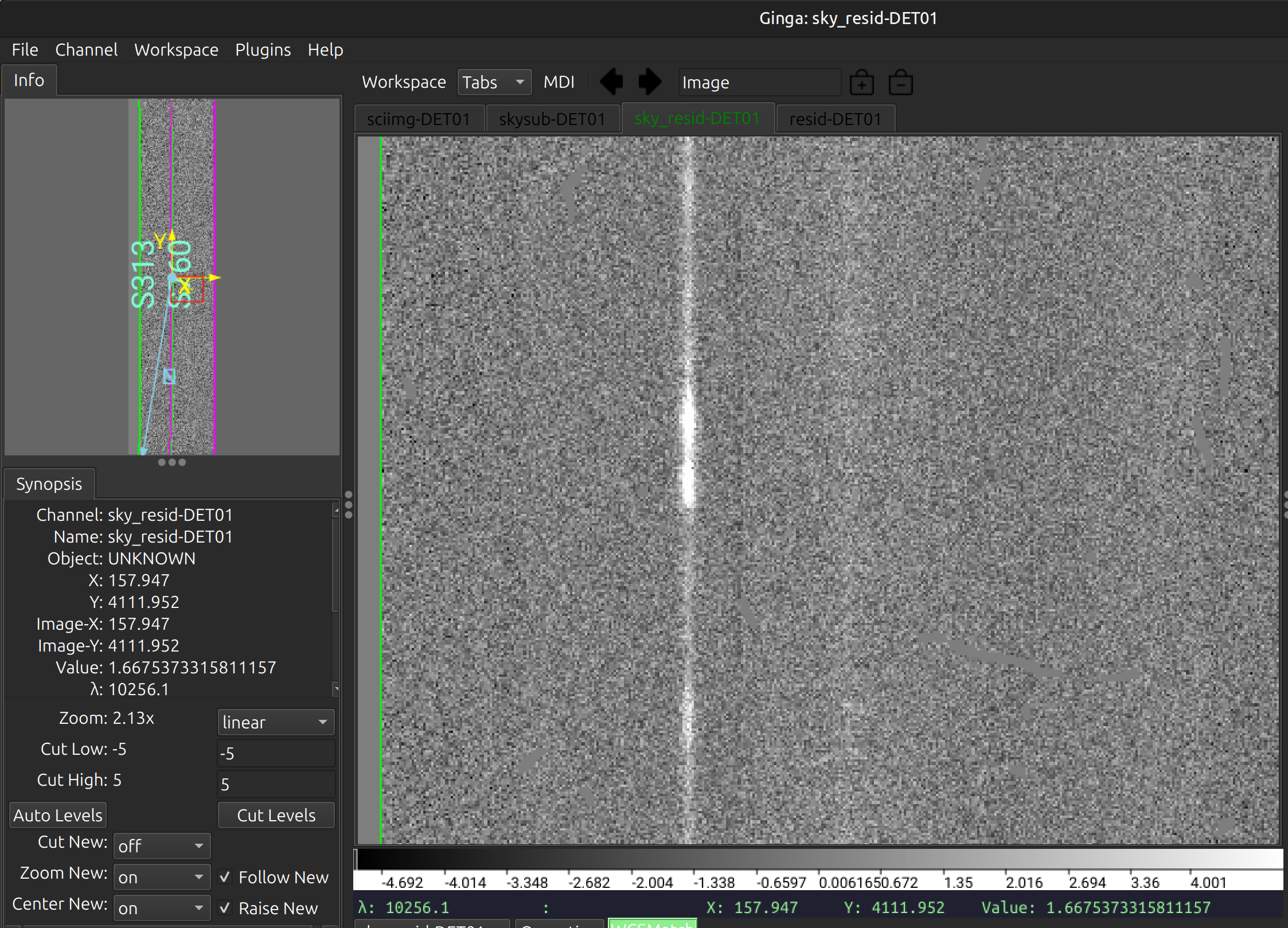
This shows on the top the calibrated science image, in the middle the sky-subtracted calibrated image, and on the bottom the sky residual image (sky-subtracted calibrated image divided by the uncertainties). The green/magenta lines are the slit edges. The orange lines (shown only in the first channel) are the object traces. See Spec2D Output for further details.
The main assessments to perform are to make sure that the object is well traced,
that there are little to no strong sky residuals in the sky_resid channel,
and that the data in the resid channel looks like pure noise (see also pypeit_chk_noise_2dspec).
Spec1D
You can see a summary of all the extracted sources in the spec1d*.txt files saved
in the Science/ folder. For this example, here are the first few lines of the file
Science/spec1d_FCSA00216334-SN2019muj_FOCAS_20201121T083826.517.txt:
| slit |                    name | obj_id | spat_pixpos | spat_fracpos | box_width | opt_fwhm |  s2n | wv_rms |
|  760 | SPAT0634-SLIT0760-DET01 |    634 |       634.2 |        0.249 |      3.00 |    0.805 | 2.14 |  0.231 |
|  760 | SPAT0700-SLIT0760-DET01 |    700 |       699.6 |        0.380 |      3.00 |    3.944 | 1.37 |  0.231 |
It shows a table with the PypeIt names of the extracted spectra in each slit and all the associated information about the extraction and the object. See Extraction Information for a detailed description of this file. Note that the maskdef_id, objname, objra, objdec and maskdef_extract columns are not printed for long-slit observations.
To inspect the 1D spectrum, we can use the script pypeit_show_1dspec, with a call like this:
pypeit_show_1dspec Science/spec1d_FCSA00216334-SN2019muj_FOCAS_20201121T083826.517.fits
which plots the spectrum in a tab of the ginga viewer and allows to select the different extracted spectra using a drop down menu, in addition to selecting other properties of the spectrum. Here is one exemple:
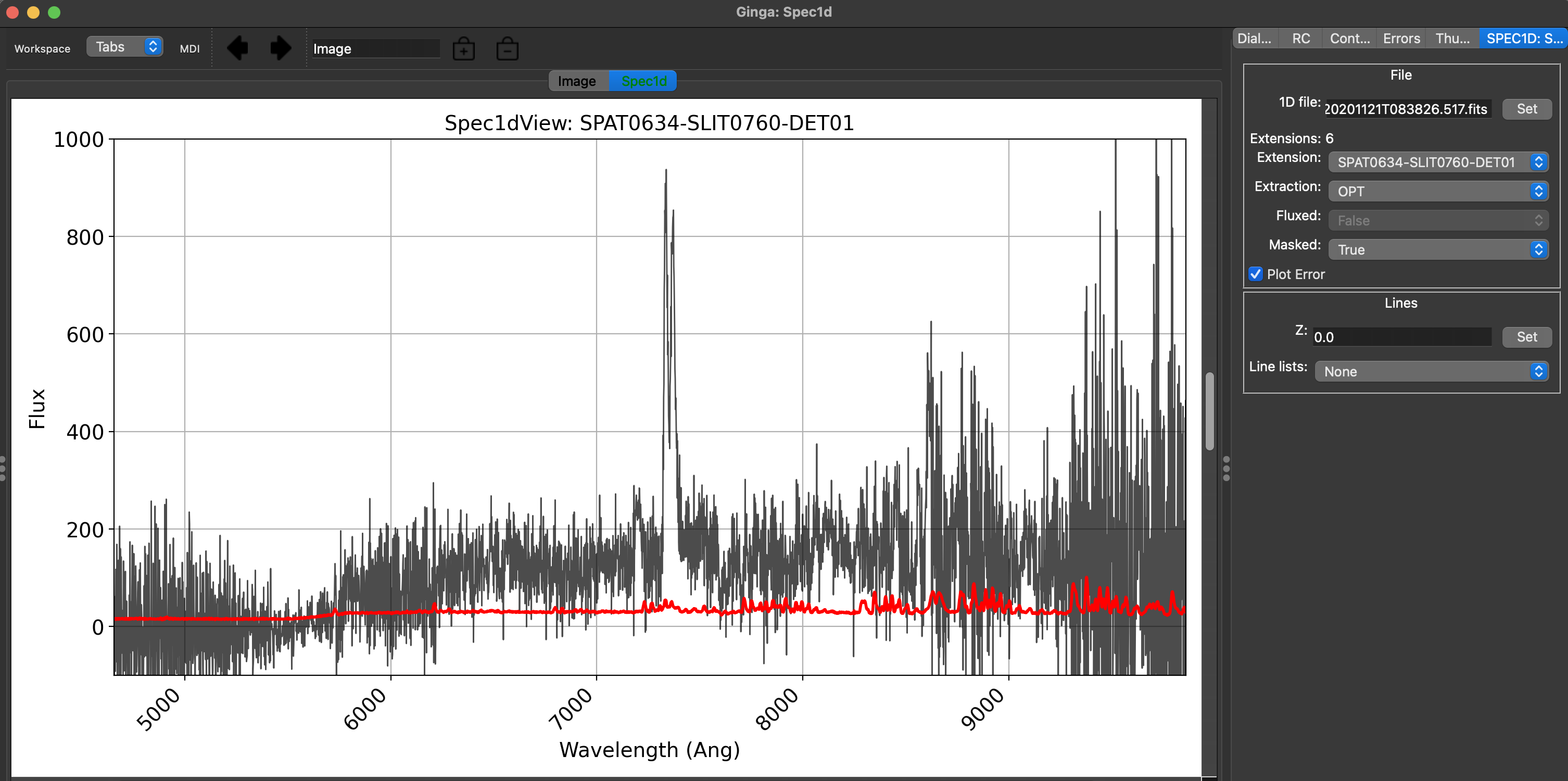
The black line is the flux and the red line is the estimated error. In the ginga window, the user can
select the different extracted spectra, the extraction type (OPT or BOX), fluxed or not fluxed spectrum, and
if showing masked data, by using the drop down menu on the right of the window. Common spectral features
can be over-plotted by selecting an option in the Line lists drop down menu and providing a redshift.
See Spec1D Output for further details.
Noise
Another important QA is to inspect the noise properties of the reduced 1D and 2D spectra.
2D
Use the script pypeit_chk_noise_2dspec to inspect the noise properties of the 2D spectra:
pypeit_chk_noise_2dspec spec2d_FCSA00216334-SN2019muj_FOCAS_20201121T083826.517.fits
This launches a GUI on your screen. Here is an example screenshot:
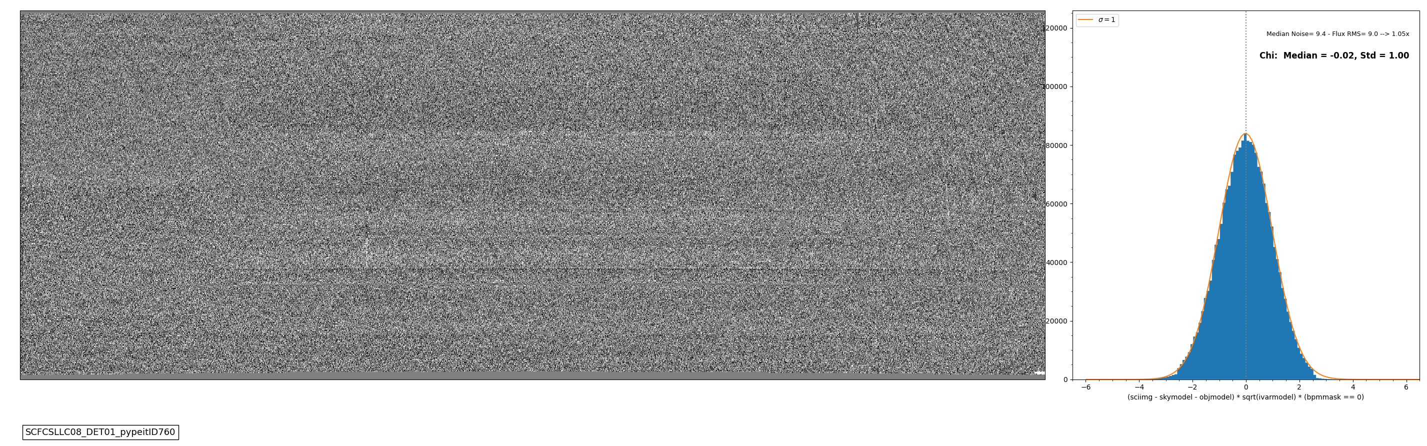
Here, we see the residuals are well centered around zero, and the histogram of the S/N values is well matched to the expected Gaussian distribution with unit variance.
1D
Use the script pypeit_chk_noise_1dspec to inspect the noise properties of the 1D spectra.
pypeit_chk_noise_1dspec spec1d_FCSA00216334-SN2019muj_FOCAS_20201121T083826.517.fits --ploterr
This launches a GUI on your screen. Here is an example screenshot:
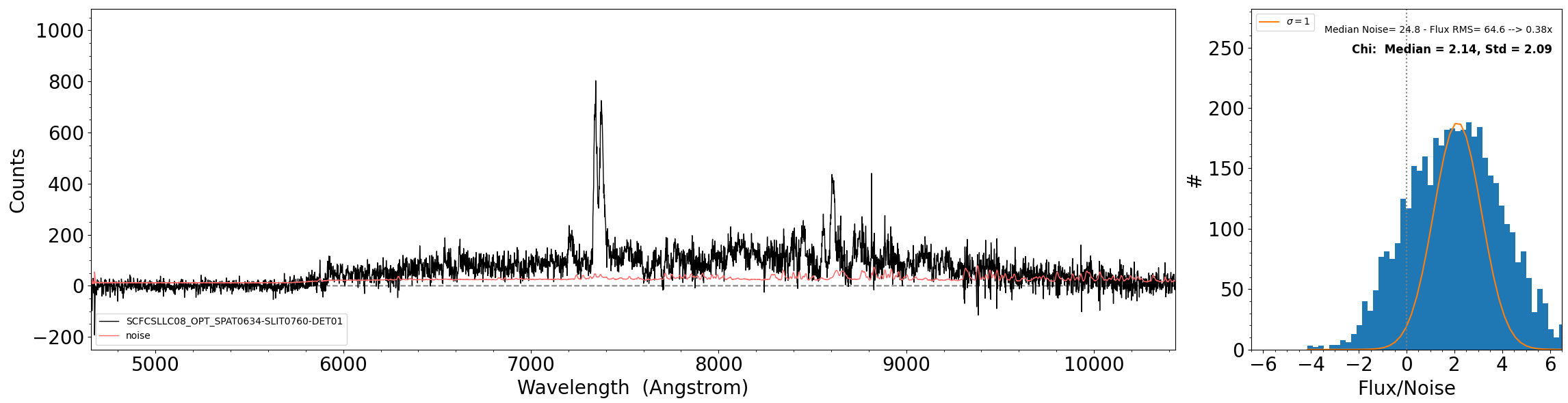
The plot on the right is showing the distribution of Flux/Noise of the extracted spectrum. In this example there is clearly flux coming from the object that biases the Flux/Noise diagnostic plot. However, this script provides the possibility to select a region in the spectrum without emission to be used for the diagnostic plot.