LDT DeVeny
Overview
This page provides a detailed outline of using PypeIt with data from the LDT/DeVeny spectrograph, including pipeline setup, parameter modifications, and troubleshooting.
Contents
The Instrument
The Lowell Discovery Telescope (LDT) is a 4.3m telescope owned by Lowell Observatory (Flagstaff, AZ) and located at a dark-sky site in northern Arizona near Happy Jack. The facility was built as the Discovery Channel Telescope, and had first light in 2012. The telescope can host up to 5 instruments simultaneously at its Cassegrain focus with fast (several minutes) switches between instruments during the night.
The DeVeny spectrograph was built at Kitt Peak National Observatory (KPNO) and was known as the White Spectrograph. It had a long career at the #1 36-inch and 84-inch telescopes there before being retired. Lowell Observatory acquired the spectrograph from KPNO on indefinite loan in 1998 and renamed the instrument in honor of the longtime KPNO Instrument Support Scientist Jim DeVeny (see a photo of DeVeny with the spectrograph on the 84-inch telescope). A new CCD camera was built for it, and the spectrograph was further modified for installation on the 72-inch Perkins telescope in 2005. Following 8 years of service there, it was removed in 2013 for upgrades for installation on the Lowell Discovery Telescope (LDT) instrument cube (see image below). DeVeny has been in service at LDT since February 2015. The spectrograph was designed for and operates internally with f/7.5 optics; new re-imaging optics were designed and fabricated to match the spectrograph with LDT’s f/6.1 beam.
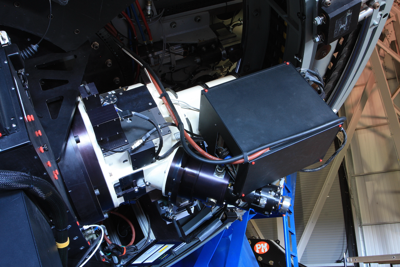
The DeVeny spectrograph mounted on one of the large side ports of the LDT instrument cube. The instrument is the white cylinder, with various electronics boxes mounted to the side and the (black-anodized) CCD camera dewar and cooler seen at a 45\(^\circ\) angle the main instrument.
EMI Pickup Noise
See the LDT Observer Tools package documentation for information about the EMI pickup noise seen in the DeVeny detector since approximately 2019.
Using PypeIt with the LDT/DeVeny Spectrograph
The LDT/DeVeny configuration parameters described herein are included
with PypeIt v1.15.0 and later[1], and the released package may be
installed via your favorite method. See the installation
instructions for steps.
Once you have installed the package, test to be sure the main driver script runs. Go to a directory outside of the PypeIt directory (e.g., your home directory) and run the main executable:
cd
run_pypeit -h
This should fail if any of the required dependencies are not satisfied. See the installation instructions for troubleshooting.
PypeIt Parameter Modifications for Specific Cases
There are various situations in which you will need to modify the Parameter Block of your PypeIt Reduction File. The default DeVeny parameters were chosen to cover the major use cases for the spectrograph, but the instrument’s high configurability and varied uses means there will still be many instances where these instrument-wide parameters must be modified. The principal categories of modifiable parameters for DeVeny users are grouped below, but the complete PypeIt list is given at User-level Parameters.
Tip
Think of parameter modifications as part of an outline, where each level represents a unique thought. Therefore, if you need to modify both the list of arc lamps and the FWHM of the arc lines under wavelength calibrations, you would include something like:
[calibrations]
   [[wavelengths]]
      lamps = HgI,CdI,ArI
      fwhm = 7.0
rather than two individual blocks. In short, each parameter group in brackets should appear only once in your Parameter Block. Also, indentation is not necessary but may help in visually organizing the outline.
Wavelength Calibration Parameters
Arc Lamps
PypeIt is able to read the identification of the energized arc lamps directly
from the DeVeny FITS header, and the user is not generally required to specify
which line lists should be used in the wavelength calibration process. There
are, however, cases where such specification is useful or necessary: a) when
the user wishes to restrict the list of lines PypeIt should consider when
creating a wavelength solution, and b) when frames taken with different lamps
are combined to create an Arc Calibration frame.
The first case should only be necessary at present for the DV4 and DV8
gratings, which rely upon the Holy Grail wavelength calibration
method. In some cases, however, including the line lists from all energized
lamps in the matching can produce spurious results (e.g., using the Hg or Cd
lists with very red spectra, or the Ne list with very blue spectra). For
example, say you energized all four DeVeny lamps when taking arc-line spectra
with DV8, centered around 8000\(\mathring{A}\). Especially if the first pass of
run_pypeit fails to produce a workable wavelength solution, you may want to
restrict the lists for matching to only Ne and Ar via:
[calibrations]
   [[wavelengths]]
      lamps = NeI_DeVeny,ArI_DeVeny
Note
As of v1.15.0, PypeIt includes instrument-specific line lists for all
four DeVeny lamps, indicated by the appended “_DeVeny” in the lamp name.
These lists have been vetted against DeVeny spectra to include lines seen
with our lamps and excluding lines not reliably detected. To specify the
PypeIt-default line lists, you may do so with the above Parameter Block
addition, using just the ion name (e.g., NeI or ArI).
For the second case, the combined Calibration frame will not combine the FITS
keywords from the input frames to produce the complete list of lines, so the
user must manually specify them. Additionally, the individual frames must be
continuum-subtracted in order to properly clip and combine the spectra into a
sensible Calibration frame. Suppose you wish to combine single-lamp frames of
Ar and Hg to create your Arc Calibration frame. You would need to add the
the following to your Parameter Block:
[calibrations]
   [[wavelengths]]
      lamps = HgI_DeVeny,ArI_DeVeny
   [[arcframe]]
      [[[process]]]
         subtract_continuum = True
   [[tiltframe]]
      [[[process]]]
         subtract_continuum = True
The order of the lamps specified here is not important, as the code sorts the list internally.
Wavelength Calibration Method
For all gratings except DV4 and DV8, template arc spectra using the Hg, Cd, and Ar lamps are included with PypeIt for use with the Full Template wavelength calibration method. If you are using one of the these gratings and relying primarily upon Ne for your calibration, it is advisable to employ the Holy Grail calibration method instead. Do so by adding the following to your Parameter Block:
[calibrations]
   [[wavelengths]]
      method = holy-grail
If both the built-in and methods fail to provide an accurate wavelength calibration, you must manually identify lines and create a template for use with that night’s data. This process is described in Troubleshooting: When Wavelength Calibration Fails.
Line Width for Arc Frames
For wavelength calibration, PypeIt assumes that your spectral line FWHM are
around 3.0 pixels (optimum value), but also measures the FWHM directly from the
Arc image. If you are using arcs taken with a slit width that produces FWHM
significantly different from this value, you may need to specify the expected
value in your PypeIt Reduction File based on a manual inspection of the arcs.
For instance, if you set the slit width to have arc lines with a FWHM of ~9
pixels (say, a 3” slit with DV1), you would specify:
[calibrations]
   [[wavelengths]]
      fwhm = 9.0
      fwhm_fromlines = False
Specifying fwhm_fromlines = False forces the code to use the supplied FWHM
and may result in a more successful wavelength calibration.
Wavelength Solution Order
Once the lines have been identified, PypeIt iteratively fits a Legendre polynomial series between pixel and wavelength space. For DeVeny, the polynomial order of the initial guess and final solution at the wavelength calibration are grating-dependent, given the varying wavelength coverages of DeVeny’s grating complement. Shown in the table below are the default values for these orders for each grating based on manual inspection of wavelength solutions.
Grating |
|
|
|---|---|---|
DV1 |
3 |
5 |
DV2 |
3 |
5 |
DV3 |
3 |
5 |
DV4 |
2 |
4 |
DV5 |
2 |
4 |
DV6 |
2 |
4 |
DV7 |
2 |
4 |
DV8 |
2 |
4 |
DV9 |
2 |
4 |
If you are unsatisfied with the RMS of the wavelength solution, adjusting the solution order may improve the situation. These values may be changed by modifying the parameters:
[calibrations]
   [[wavelengths]]
      n_first = <initial guess>
      n_final = <final solution>
Here, n_first is the initial order used in the iterative solution (this may
need modification if a holy-grail attempt fails), and n_final is the
final order of the solution (this may be modified to alter the RMS of the wavelength solution).
Night Sky Lines for Calibration
Use of night sky lines for wavelength calibration is the basis of DeVeny’s
Flexure Correction (see Special Consideration: Flexure in DeVeny and How PypeIt Handles It). You will need to take at least
one arc spectrum at some point in the night (e.g., during start-of-night
calibrations) to establish a wavelength reference across the CCD. PypeIt
extracts the night sky spectrum from the background of your science frames,
and computes an approximate wavelength calibration by cross-correlating it
with an archived sky spectrum. No additional arcs are needed to make this
link, and PypeIt will compute a pixel shift in the wavelength calibration to
match your science frame with your Arc. No changes to the Parameter Block
of your PypeIt Reduction File are required, as this is the default behavior for
DeVeny data.
PypeIt does support night-sky wavelength calibration for near-infrared instruments using the copious OH lines in this portion of the spectrum, but DeVeny does not reach far enough into IR for this method to provide useful wavelength solutions.
Object Finding and Extraction
The parameters related to object finding and extraction are generally modified
after you have done an initial pass through run_pypeit, and you wish to
improve the ability of the code to work with your data.
General Object Finding
Refer to the Object Finding documentation for full details on the
algorithms. Object finding is governed by the findobj set of parameters,
and is carried out on the spectrally-smashed image. PypeIt produces a quality
assurance plot for object finding on each 2D spectral image (shown below for
the example frame used in this document).
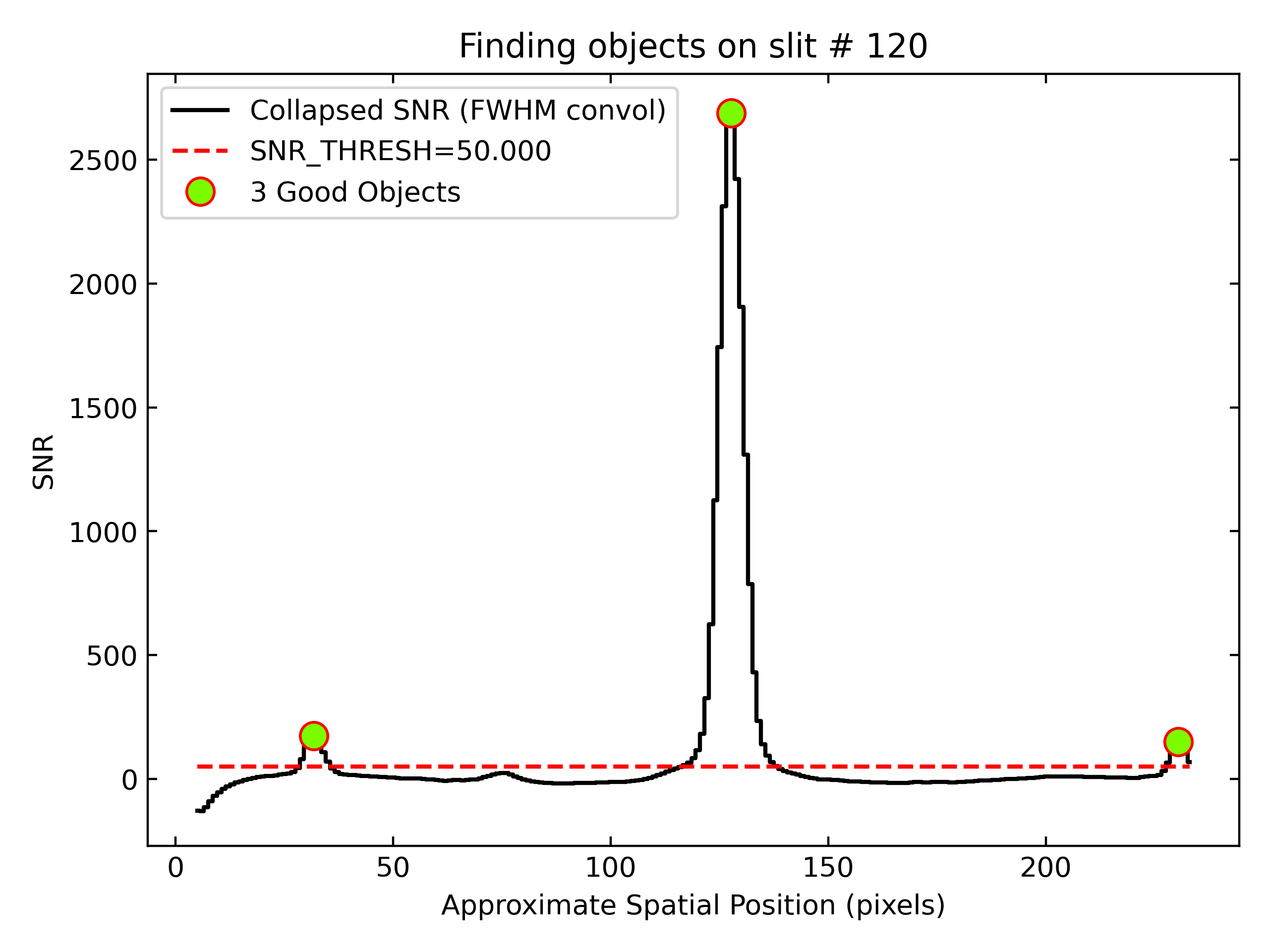
Example of PypeIt object finding QA for the 2D spectral image shown above,
where the black plot is the spectrally summed spatial distribution of
signal-to-noise in the image. The red dashed line indicates the
snr_thresh parameter, which can be adjusted to either allow other peaks
in the plot to “surface” or to “submerge” unwanted objects.
The most commonly modified parameter is snr_thresh, which limits the search
to sources with peak flux in excess of the threshold times the RMS of the
smashed image. The default is S/N = 50, but you may wish to modify this
parameter to find more/fewer objects. For instance, if you wish the code to
automatically find fainter objects with peak flux 10\(\sigma\) above the estimated RMS
in the integrated slit profile, you would add the following to the Parameter
Block:
[reduce]
   [[findobj]]
      snr_thresh = 10.
On the flip side, if you observed fairly bright objects and want to eliminate
the inclusion of spurious faint sources in your final spec1d file, you may
increase snr_thresh to the point that only a single object is detected.
Similarly, you could use the parameter maxnumber_sci to limit the object
finding to a specified number of objects in each science frame (ordered by
flux):
[reduce]
   [[findobj]]
      maxnumber_sci = 1
Nights with Poor (or Really Excellent) Seeing or Observations of Extended Objects
The default initial object finding kernel size for DeVeny data assumes a seeing
of ~1.5” regardless of binning[5], which should cover most conditions at LDT
when observing pointlike objects. If the seeing is significantly better or
worse than this value – or you are observing extended objects – and you are
having difficulty automatically finding your desired objects in the frame, you
may alter the value with the find_fwhm parameter. Note that this parameter
is specified in pixels rather than arcseconds (the default value is 4.4
pixels for unbinned data). Compute the needed value via:
For instance, if you had 2.5” seeing with unbinned data, you would specify:
[reduce]
   [[findobj]]
      find_fwhm = 7.4
A related parameter you may need to modify is the radius around the peak of the trace to use for boxcar extraction of the source, which is specified in arcseconds. The DeVeny default value is 1.9” (for a total boxcar width of 3.8” centered on the trace). You will want this parameter to be ~1.3x the seeing to encompass nearly 100% of the flux assuming a Gaussian profile. So, for the aforementioned 2.5” seeing, you should specify:
[reduce]
   [[extraction]]
      boxcar_radius = 3.2
in your PypeIt Reduction File.
Warning
Unlike find_fwhm, boxcar_radius is specified in arcseconds, which
is unaffected by CCD binning.
All of the above applies equally well to nights with exceptional seeing (\(\leq\)0.8”), where tightening up these parameters might be necessary to properly find and extract your spectra or to extended objects whose profiles along the slit are much wider than the seeing disk.
Extraction with Extended Emission Lines
It is common for bright emission lines to spatially extend beyond the source continuum, especially for galaxies or comets. In these cases, the code may reject the emission lines because they present a different spatial profile from the majority of the flux. While this is a desired behavior for optimal extraction of the continuum, it leads to incorrect and non-optimal fluxes for the emission lines.
The current mitigation is to allow the code to reject the pixels for profile estimation but then to include them in extraction. This may mean the incurrence of cosmic rays in the extraction. To utilize this strategy, add the following to the Parameter Block:
[reduce]
   [[extraction]]
      use_2dmodel_mask = False
It is likely that you will want to use the BOXCAR extractions instead of the
OPTIMAL, but caveat emptor. When viewing the 2D spectrum using the
pypeit_show_2dspec script, you should use the --ignore_extract_mask
option.
For very extended, bright emission lines you may need to additionally use:
[reduce]
   [[skysub]]
      no_local_sky = True
to avoid poor local sky subtraction. See the Sky Subtraction documentation for
further details. Note that if this option is used, no object model will be
created or saved (the object will be extracted) and the output of
pypeit_show_2dspec will not look as clean as that shown above.
Emission Line Only or High-\(z\) Objects
If you have a faint object with only emission lines or a high-\(z\) object that only appears on part of the trace, you may need to specify the spectral range on the CCD over which the pipeline should search for the object. Do this with:
[reduce]
   [[findobj]]
      find_min_max = minpixel, maxpixel
where minpixel and maxpixel are the spectral pixels bounding the
region you see your object in the 2D spectra as inspected with
pypeit_show_2dspec. By limiting the spectral range over which the object
finding happens, the S/N in the smashed image will be improved and the code may
be able to more easily identify the object. If this step doesn’t work, then
proceed with manual extraction as described in Missing 1D Spectra.
Observations at High Airmass
Because of LDT’s ability to point to low elevation angles, many observers procure science frames taken at high airmass. Pointlike objects will then smear out into a rainbow (and look like cigar-shaped objects along the parallactic angle in the slit viewer). Aligning the slit with this elongation allows all light from the object to pass into the spectrograph, but will end up with a curved trace on the detector with respect to the slit edges.
For instance, the spectrum below was taken with the DV1 (150 l/mm) grating.
Shown are the spec2d file and Object Tracing QA plot for an object
observed at an elevation of 11\(^\circ\) above the horizon (airmass 5).

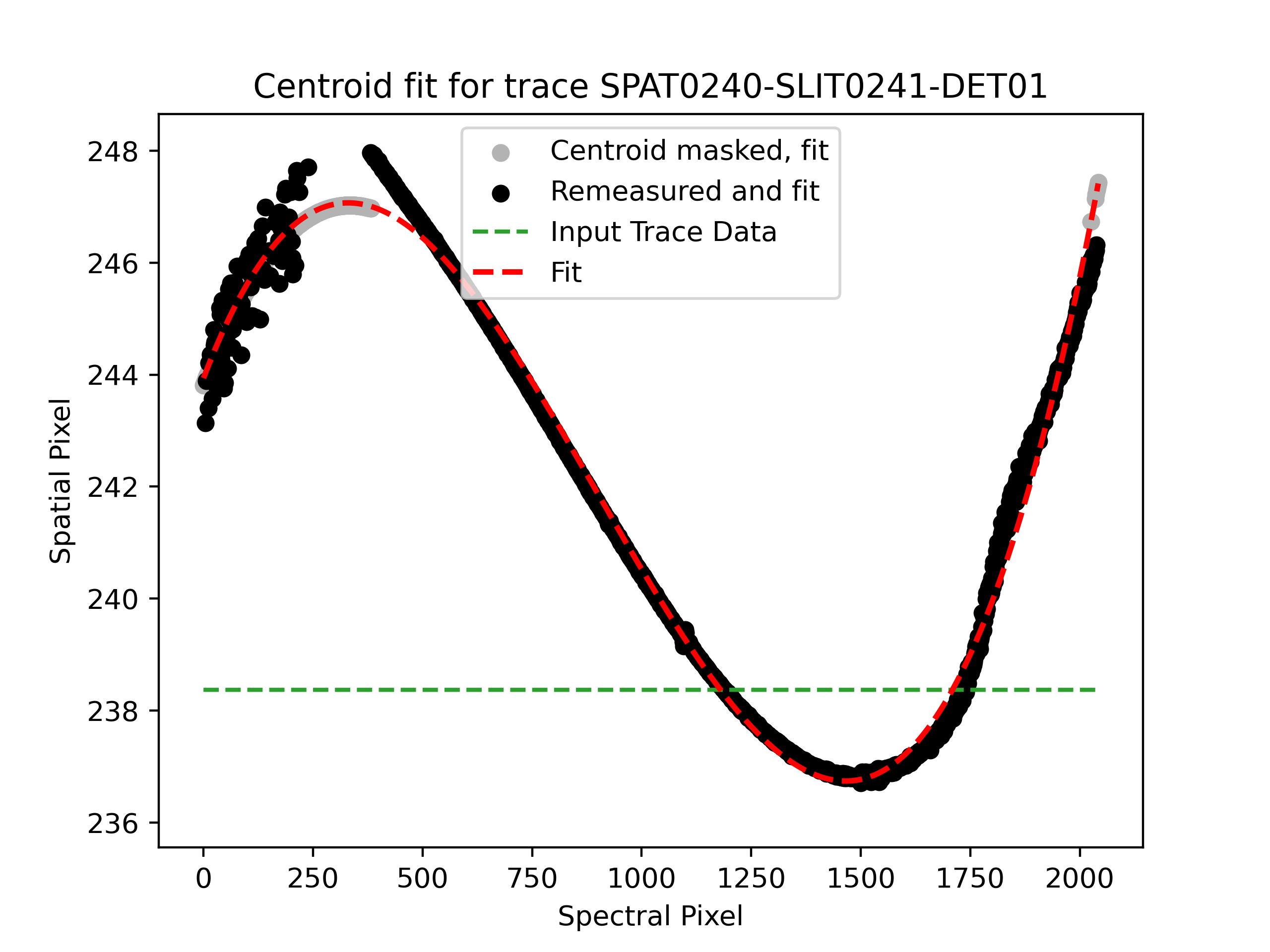
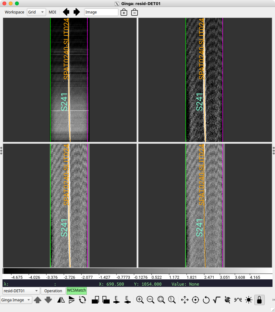
Initial poor object tracing for this high-airmass object. The left
panel shows the spec2d ginga window, and the right panel shows the
QA plot.
The tracing algorithm was not able to follow the curve of the spectrum to
larger spatial pixel (rightward in the spec2d image) at low spectral pixel
(low wavelength), and instead tried to grab onto peaks in the noise closer to
the “Input Trace Data” (parallel to the slit edge). In cases like this, you
may need to allow PypeIt to follow traces further from the line defined by the
slit edges. The parameter trace_maxshift (default value = 2 pixels for
DV1) may be increased incrementally to allow the curved spectrum to be traced.
By using the following combination of parameters, the object tracing algorithm
is now able to trace the object cleanly across the entire spectral image, as
shown in the panels below below.
[reduce]
    [[findobj]]
        trace_maxshift = 3.0
        trace_npoly = 4
        find_numiterfit = 100
        find_min_max = 900,1700
        trace_min_max = 100,1700
The parameter find_min_max = 900,1700 directs PypeIt to only spectrally
smash the image over the range from pixel 900 to pixel 1700 (useful if the
spectral trace fades at the ends of the detector), and trace_min_max =
100,1700 indicates that all pixels outside of this range should be masked
when fitting the object trace (useful for similar reasons as above). In the
lower plot, the masked ranges are visible as the light blue regions at the
upper and lower spectral ends.
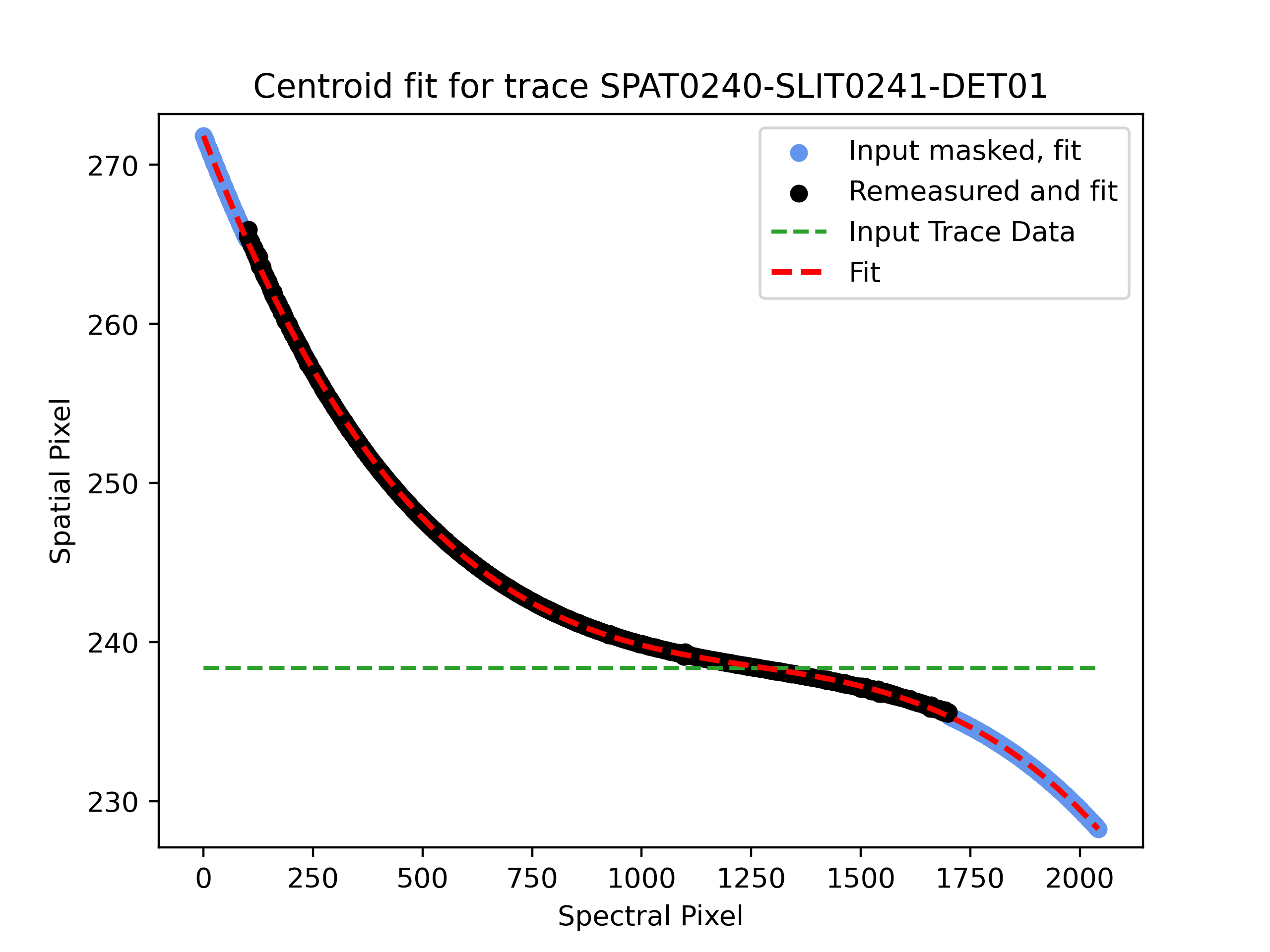
Improved object tracing for this high-airmass object using the adjusted
PypeIt parameters listed above. The left panel shows the spec2d
ginga window, and the right panel shows the QA plot.
Not only does the trace now follow the blue end (low spectral pixel number), but it is monotonic in spatial pixel space, as mandated by the physics of atmospheric refraction. See the Object Tracing QA documentation for more details on the interpretation of this plot.
Miscellaneous Parameters
Illumination Correction
If your science program requires correcting for the illumination pattern along the slit, it is possible to turn on this function. Flexure in the spatial direction is not yet accounted for, and a shifted illumination function correction can introduce systematic error into extracted spectra. If your science program requires illumination correction for variations in throughput along the slit, you may do so using either dome flats or sky flats and adding the following to the Parameter Block of your PypeIt Reduction File:
[baseprocess]
   use_illumflat = True
Twilight sky flats (identified as such in the LOUI) will automatically be
labeled with frame type illumflat, but if you wish to use dome flats for an
illumination correction, you will need to add this frame type to your dome
flats in the Data Block of your PypeIt Reduction File.
Beyond the Red
If your spectra are exclusively in the very red end of the DeVeny range (\(\lambda \gtrsim 7000 \mathring{A}\)), and you are flux calibrating your data, you will need to correct for telluric absorption (at wavelengths below this value, the UVIS extinction model is used for the sensitivity function). You must specify the IR algorithm when creating the sensitivity function to correctly account for atmospheric absorption in this range of the spectrum. See the Telluric Correction documentation for current practices.
Special Considerations, Advanced Usage, and Troubleshooting
Special Consideration: Flexure in DeVeny and How PypeIt Handles It
The standard method for flexure correction in the DeVeny camera is to apply a shift based on the extracted sky spectrum during the main PypeIt run. This method is applied automatically using the current DeVeny parameters, and you should use only single-pointing arcs for wavelength calibration (e.g., taken at zenith or the position of the flatfield screen).
This method of flexure correction computes a cross-correlation between the extracted sky spectrum and an archived spectrum (currently the sky above Cerro Paranal). To use a different sky spectrum, specify (e.g., for the Mt. Hamilton, CA spectrum shown below):
[flexure]
   spectrum = sky_kastb_600.fits
The computed correlation is used to shift the wavelength solution in pixel space to align with the night sky lines extracted from the 2D image via simple linear interpolation. Examples of the quality assurance plots for this process are shown below.
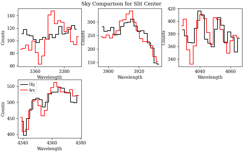
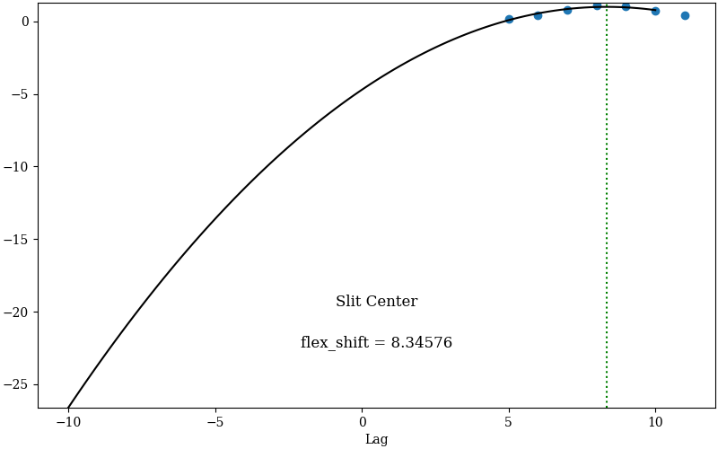
Example of PypeIt flexure QA for a science frame of BD+28 4211. Left:
Plots of selected spectral lines for the science frame (black) and
archived sky spectrum above Mt. Hamilton, CA (red). Right: The
cross-correlation between the red and black sky spectra (blue dots) and a
parabolic fit (black) for determining the location of maximum correlation
(”flex_shift”).
If you wish to have no flexure correction applied, you may specify the following:
[flexure]
     spec_method = skip
If your science requirements indicate the taking of in situ arcs for
wavelength calibration, see Advanced Usage: Calibration Groups for a description of this
advanced usage. In this case, you may want to set spec_method = skip,
otherwise flexure corrections will still be applied. It may be instructive to
see the magnitude of the flexure correction with in situ arcs, which should
be well under a pixel.
Advanced Usage: Calibration Groups
By default, PypeIt will use all calibration frames within a given setup
(e.g., A) for all science frames within that setup. For many DeVeny
programs, this is perfectly acceptable. It is possible, however, to assign
particular calibration frames to specific science frames as required by the
science program.
PypeIt uses the concept of a “calibration group”
to define complete sets of calibration frames (e.g., arcs, flats, biases) and
the science frames to which these calibration frames should be applied. The
necessary calib column is already included in the PypeIt Reduction File
produced by pypeit_setup, and all that is necessary is to adjust the values
there according to your requirements. For example, say we wanted to
(arbitrarily) assign some science frames to the first arc and flat (group 1),
some to the first arc and last flat (group 2), and some to the last arc and
last flat (group 3). You would edit the calib column of the .pypeit
file to look something like this:
# Data block
data read
path /data/20210522a
          filename |       frametype | ... |filter1 | slitwid | lampstat01 | calib
20210522.0057.fits |        arc,tilt | ... |  CLEAR |     1.1 | Cd, Ar, Hg |   1,2
20210522.0058.fits |        arc,tilt | ... |  CLEAR |     1.1 | Cd, Ar, Hg |     3
20210522.0001.fits |            bias | ... |  CLEAR |     1.1 |        off |   all
20210522.0002.fits |            bias | ... |  CLEAR |     1.1 |        off |   all
...
20210522.0032.fits |       illumflat | ... |  CLEAR |     1.1 |        off |   all
20210522.0033.fits |       illumflat | ... |  CLEAR |     1.1 |        off |   all
...
20210522.0022.fits | pixelflat,trace | ... |  CLEAR |     1.1 |        off |     1
20210522.0023.fits | pixelflat,trace | ... |  CLEAR |     1.1 |        off |     1
20210522.0024.fits | pixelflat,trace | ... |  CLEAR |     1.1 |        off |   2,3
20210522.0025.fits | pixelflat,trace | ... |  CLEAR |     1.1 |        off |   2,3
...
20210522.0078.fits |         science | ... |  CLEAR |     1.1 |        off |     1
20210522.0079.fits |         science | ... |  CLEAR |     1.1 |        off |     1
20210522.0080.fits |         science | ... |  CLEAR |     1.1 |        off |     2
20210522.0081.fits |         science | ... |  CLEAR |     1.1 |        off |     2
20210522.0082.fits |         science | ... |  CLEAR |     1.1 |        off |     3
20210522.0083.fits |         science | ... |  CLEAR |     1.1 |        off |     3
data end
You may assign calibration frames to one or more groups via comma-separated
lists or the “all” specifier. Science frames, however, must belong to one
and only one calibration group.
This division of frames could be useful if the observer takes both evening and
morning calibration frames (and wished to associate certain science frames with
one set or the other), or requires the use of in situ arcs for wavelength
calibration. After successfully processing the calibration frames, the code
will write out a .calib file that specifies which calibration frames have
been assigned to each calibration group. It will be important to inspect this
file before proceeding with the full reduction to ensure everything is grouped
as expected.
Whether or not you choose to use calibration groups, PypeIt will include in the
FITS HISTORY cards (of the spec2d and spec1d files) the list of
calibration frames used to process each science image.
Troubleshooting: Crash on improper frame types
If your PypeIt run crashes out very early (i.e., just after reading in the frame metadata), and you get output to your screen similar to:
[INFO]    :: metadata.py 1287 get_frame_types() - Typing files
[INFO]    :: metadata.py 1297 get_frame_types() - Using user-provided frame types.
[ERROR]   :: bitmask.py 112 _prep_flags() - The following bit names are not recognized: None
[ERROR]   :: metadata.py 1303 get_frame_types() - Improper frame type supplied!
            Check your PypeIt Reduction File
Traceback (most recent call last):
...
    raise PypeItError(msg)
pypeit.pypmsgs.PypeItError: Improper frame type supplied!
            Check your PypeIt Reduction File
the issue is the inclusion of files with a frametype of None in your
PypeIt Reduction File. Go back to Edit Your PypeIt File and verify all files
listed in your PypeIt Reduction File meet the criteria described therein.
As of v1.14.0, PypeIt automatically comments out lines in the Data Block
with a frametype of None, greatly easing headaches related to this
issue.
Troubleshooting: When Wavelength Calibration Fails
The trickiest piece with spectroscopic data reduction is the production of a
valid wavelength calibration. PypeIt produces Quality Assurance plots of this
step for inspection, and you may use the pypeit_chk_wavecalib script to
determine the accuracy of the calibration. Shown below are QA/ examples of
both accurate and poor wavelength calibrations.
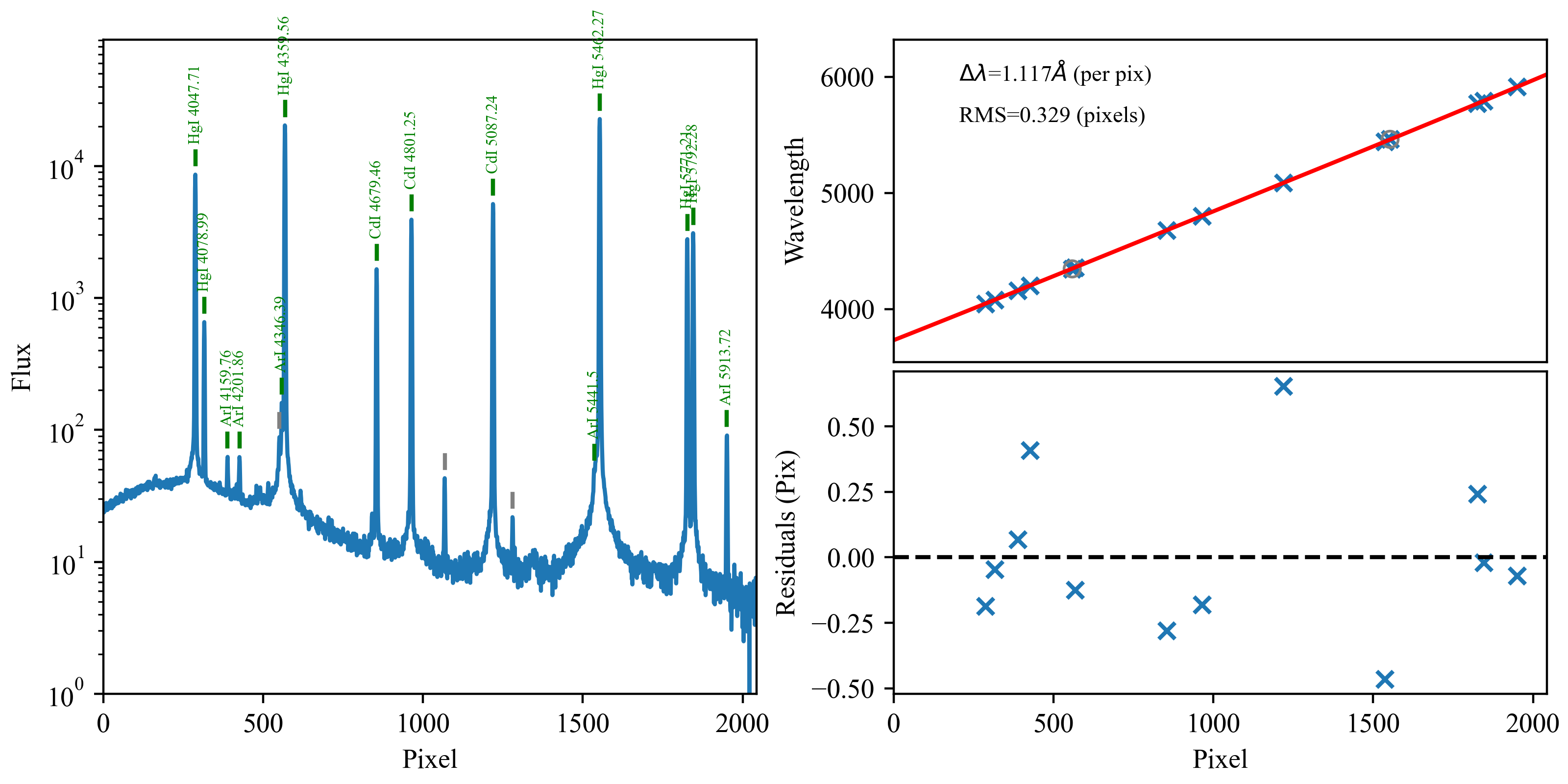
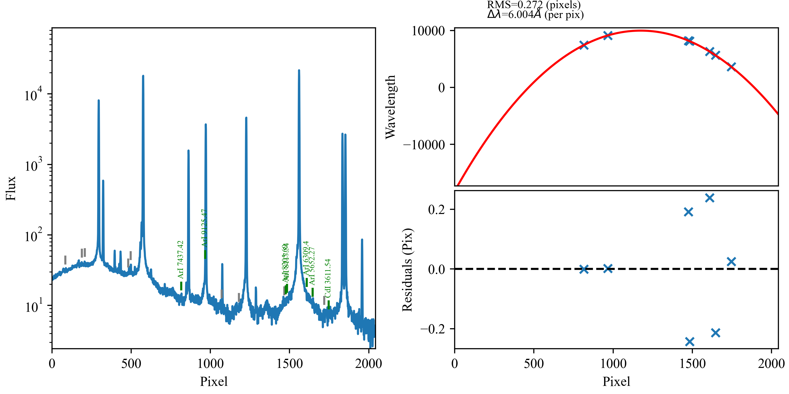
Examples of good (top) and not-so-good (bottom) wavelength
calibrations for the same setup using DV6 on different nights. For the
top plots, PypeIt found the bright lines, correctly associated them with
the line lists, and produced a roughly linear wavelength as a function of
pixel number. In the bottom plots, the holy-grail method was not able
to correctly identify the lines, latching onto noise in the continuum,
and produced a nonsensical wavelength solution.
As of v1.9.0, PypeIt contains full wavelength templates for the 150g/mm
(DV1), 300g/mm (DV2, DV3), 600g/mm (DV6, DV7), and 1200g/mm (DV9) gratings,
with a more complete template for the 500g/mm (DV5) grating added in
v1.15.0. The code uses the full_template method to match your arc
spectrum against the template using a cross-correlation to establish the
wavelength baseline for identifying and fitting individual lines. These
templates were created using the Hg, Cd, and Ar lamps – if your particular
data sets do not match this lamp set, the cross correlation may not work as
nicely, and you could end up with a situation such as shown in the right panel
above. For gratings DV4 and DV8, we do not yet have good template spectra, and
so these gratings rely upon the holy-grail method based on pattern matching
the detected lines with that expected from the lamps observed. If you take arcs
with these gratings, please let LDT staff know so that our template archive can
grow.
While examining the calibration outputs from run_pypeit -c
(Examine the Calibration Files), if you find either a wavelength calibration akin
to the bottom plots above or no wavelength calibration at all, the calibration
has failed. If adjusting wavelength calibration parameters
(Wavelength Calibration Parameters) does not resolve the issue, the most efficient way
forward is to manually identify the lines using the By-Hand Approach of
pypeit_identify and the reference spectra in the DeVeny User Manual. Since
v1.9.0, PypeIt has the ability to cache and directly use the output of
pypeit_identify. When you save and quit the GUI, the script will print
instructions in the terminal for using the wavelength solution you just
created, namely adding the following to the parameter block of your PypeIt
Reduction File:
[calibrations]
      [[wavelengths]]
         reid_arxiv = wvarxiv_ldt_deveny_<YYYYMMDD>T<HHMM>.fits
         method = full_template
where the date and time in the filename are those of the file’s creation.
Simply add the block and run_pypeit.
If you need to do this for your data, please also send your wvarxiv.fits,
wvcalib.fits, and DeVeny setup information to LDT Staff so that it may be
added to the standard PypeIt configuration in a future release.
Troubleshooting: Other edge cases or weird crashes
If you encounter other failure modes of the pipeline, please contact LDT Staff
for troubleshooting. The most efficient method of contact is to use the
#ldt-deveny channel of the PypeIt Users Slack.
Cheat Sheet for Common DeVeny Workflows
Listed here is a brief “cheat sheet” of commands for a common DeVeny workflow for quick reference.
Set up the PypeIt Reduction File(s)
pypeit_setup -s ldt_deveny
pypeit_setup -s ldt_deveny -c <all or subset ID>
Edit the PypeIt Reduction File(s) as necessary
Run PypeIt on the calibrations and inspect
run_pypeit ldt_deveny_<subset ID>.pypeit -c
pypeit_chk_edges ...
pypeit_chk_wavecalib ...
pypeit_chk_flats ...
pypeit_identify ...
Run PypeIt on your science data
run_pypeit ldt_deveny_<subset ID>.pypeit -o
pypeit_show_2dspec ...
pypeit_show_1dspec ...
Run any desired afterburner scripts
pypeit_sensfunc ...
pypeit_flux_setup Science/
pypeit_flux_calib ...
Example PypeIt Directory Structure
This is an example of the directory structure generated by PypeIt, with
RAWDIR the as the base. In this way, both the raw and processed data files
are in the same place.
RAWDIR
├── 20290101.0001.fits
├── 20290101.0002.fits
├── ...
├── ldt_deveny_A
│ ├── Calibrations
│ │ ├── Arc_A_0_DET01.fits
│ │ ├── Bias_A_0_DET01.fits
│ │ ├── ...
│ ├── QA
│ │ ├── MF_A.html
│ │ └── PNGs
│ │     ├── Arc_1dfit_A_0_DET01_S0120.png
│ │     ├── Arc_FWHMfit_A_0_DET01_S0120.png
│ │     ├── ...
│ ├── Science
│ │ ├── spec1d_20290101.0045-3c273_DeVeny_20290101T044914.020.fits
│ │ ├── spec1d_20290101.0045-3c273_DeVeny_20290101T044914.020.txt
│ │ ├── spec2d_20290101.0045-3c273_DeVeny_20290101T044914.020.fits
│ │ ├── ...
│ ├── ldt_deveny_A.calib
│ ├── ldt_deveny_A.log
│ ├── ldt_deveny_A.pypeit
├── setup_files
│ ├── ldt_deveny.calib
│ ├── ldt_deveny.obslog
│ └── ldt_deveny.sorted