LBT/MODS HOWTO
Overview
This document provides a guide to reducing MODS longslit data with PypeIt: (1) from setting up the pypeit file; (2) through the main pypeit run which performs the wavelength calibration, sky subtraction and extraction; (3) to the final steps of flux calibration, coaddition of the extracted 1D spectra and correction of telluric absorption.
There are two sets of MODS spectrograph classes: (1) the original ones (lbt_mods1b, lbt_mods1r, lbt_mods2b and lbt_mods2r) which work on the raw 2D spectra and (2) four new ones (lbt_mods1b_proc, lbt_mods1r_proc, lbt_mods2b_proc and lbt_mods2r_proc) which were added in v1.18 and work on spectra which have been pre-processed by the modsCCDRed scripts. The modsCCDRed scripts overscan-subtract, trim, flat-field and flip the red-channel data about the Y axis. Pre-processed data will have the suffix _otf. Using modsCCDRed to pre-process the spectra, and then feeding the results into a spectroscopic data reduction pipeline, has been the standard procedure for reducing MODS data.
This tutorial will use the _proc classes, but within the RAW_DATA folder of the shared google drive, linked from this page, you can find sets of both raw and pre-processed data, and pypeit_files for each dataset are in Pypeit-development-suite github.
Setup
Organize the data
The directory of pre-processed images should contain, for each channel (e.g. MODS1/2 Red/Blue), the science and spectrophotometric standard star spectra, the set of 3 arcs and the set of slit flats taken through the science slit and the standard star slit. MODS longslit arcs always use the 0.6” wide segmented long slit; MODS spectrophotometric standards always use the 5”x60” slit; and science data may be taken through any of the segmented slits (0.3”, 0.6”, 0.8”, 1”, 1.2”, or 2.4”) or the wide 5” slit, so your directory could potentially contain spectra taken through 3 different slits. However, all of these data can be combined into a single pypeit file, and since the edges of the central segment of the science slit match those of the 5” wide slit, only the science slit flats will be used to trace the spectra. This has the advantage that the main pypeit run only needs to be done only once per channel and that the standard star trace is available for use as a crutch for tracing a science target with a weak continuum.
The MODS1 Dual Grating data on the z~3 quasar, HS1946+7658 will be used for this tutorial. In this example, the pre-processed blue and red channel data are stored in the folders:
/PypeIt-development-suite/RAW_DATA/lbt_mods1b_proc/dual_grating_longslit_qso and /PypeIt-development-suite/RAW_DATA/lbt_mods1r_proc/dual_grating_longslit_qso
The files within the lbt_mods1b_proc and lbt_mods1r_proc folders are.
FILENAME                      OBJECT INSTRUME DICHNAME MASKNAME GRATNAME EXPTIME AIRMASS
mods1b.20230909.0024_otf.fits Feige_110_dual_grating MODS1B Dual LS60x5 G400L 90.0 1.35
mods1b.20230909.0028_otf.fits HS1946+7658 MODS1B Dual LS5x60x0.8 G400L 400.0 1.96
mods1b.20230910.0028_otf.fits Ne_+_Hg_Lamps MODS1B Dual LS5x60x0.6 G400L 2.0 1.00
mods1b.20230910.0029_otf.fits Kr_+_Xe_Lamps MODS1B Dual LS5x60x0.6 G400L 15.0 1.00
mods1b.20230910.0030_otf.fits Ar_Lamp MODS1B Dual LS5x60x0.6 G400L 30.0 1.00
mods1b.20230910.0048_otf.fits QTH1_ND1.5_Dual_LS5x60x0.8_Slit_Flat MODS1B Dual LS5x60x0.8 G400L 20.0 1.00
mods1b.20230910.0049_otf.fits QTH1_ND1.5_Dual_LS5x60x0.8_Slit_Flat MODS1B Dual LS5x60x0.8 G400L 20.0 1.00
mods1b.20230910.0051_otf.fits QTH1_UG5_Dual_LS5x60x0.8_Slit_Flat MODS1B Dual LS5x60x0.8 G400L 8.0 1.00
mods1b.20230910.0052_otf.fits QTH1_UG5_Dual_LS5x60x0.8_Slit_Flat MODS1B Dual LS5x60x0.8 G400L 8.0 1.00
mods1b.20230910.0080_otf.fits QTH1_ND1.5_Dual_LS60x5_Slit_Flat MODS1B Dual LS60x5 G400L 3.5 1.00
mods1b.20230910.0083_otf.fits QTH1_UG5_Dual_LS60x5_Slit_Flat MODS1B Dual LS60x5 G400L 1.5 1.00
and
FILENAME                      OBJECT INSTRUME DICHNAME MASKNAME GRATNAME EXPTIME AIRMASS
mods1r.20230909.0044_otf.fits Feige_110_dual_grating MODS1R Dual LS60x5 G670L 90.0 1.35
mods1r.20230909.0051_otf.fits HS1946+7658 MODS1R Dual LS5x60x0.8 G670L 400.0 1.96
mods1r.20230910.0028_otf.fits Ne_+_Hg_Lamps MODS1R Dual LS5x60x0.6 G670L 1.1 1.00
mods1r.20230910.0029_otf.fits Kr_+_Xe_Lamps MODS1R Dual LS5x60x0.6 G670L 1.0 1.00
mods1r.20230910.0030_otf.fits Ar_Lamp MODS1R Dual LS5x60x0.6 G670L 1.0 1.00
mods1r.20230910.0044_otf.fits QTH1_ND1.5_Dual_LS5x60x0.8_Slit_Flat MODS1R Dual LS5x60x0.8 G670L 2.0 1.00
mods1r.20230910.0047_otf.fits VFLAT10.0_Clear_Dual_LS5x60x0.8_Slit_Flat MODS1R Dual LS5x60x0.8 G670L 2.0 1.00
mods1r.20230910.0080_otf.fits VFLAT5.0_Clear_Dual_LS60x5_Slit_Flat MODS1R Dual LS60x5 G670L 3.0 1.00
mods1r.20230910.0081_otf.fits VFLAT5.0_Clear_Dual_LS60x5_Slit_Flat MODS1R Dual LS60x5 G670L 3.0 1.00
The input files should be collected into a directory on your machine, e.g. $DATA/dual_grating_longslit_qso/Proc/ (Proc, to indicate that these are pre-processed and not raw data). You should create a separate directory, e.g. $DATA/dual_grating_longslit_qso/pypeit_rdx/ in which to run pypeit.
Run pypeit_setup
In the pypeit_rdx/ sub directory, run pypeit_setup to create the pypeit input files for the blue and red channels.
(pypeit18)% cd pypeit_rdx
(pypeit18)% pypeit_setup -r $DATA/dual_grating_longslit_qso/Proc/mods1b -s lbt_mods1b_proc -c A
(pypeit18)% pypeit_setup -r $DATA/dual_grating_longslit_qso/Proc/mods1r -s lbt_mods1r_proc -c A
This will create subdirectories lbt_mods1b_proc_A/ and lbt_mods1r_proc_A/ and write the pypeit files for the blue and red channels into their respective subdirectories.
Note
If there is more than one configuration in the Proc directory, e.g. MODS1B spectra taken in blue-only and also in dual (dichroic) modes, then -c A will choose only the first configuration. You should store blue-only, red-only and dual mode data in separate raw(processed) data directories.
Modify the pypeit setup files
Now, make the following edits to the pypeit setup files:
Remove frametypes pixelflat and illumflat from the slit flats since, in this case, they will be used only to trace the slit edges. The 20 spaces keep the columns aligned, but this is only for readability as the columns in pypeit files are separated by ‘|’ and don’t need to line up.
sed -i -e s/pixelflat,illumflat,/'\ \ \ \ \ \ \ \ \ \ \ \ \ \ \ \ \ \ \ \ '/ lbt_mods1b_proc_A.pypeit

sed -i -e s/pixelflat,illumflat,/'\ \ \ \ \ \ \ \ \ \ \ \ \ \ \ \ \ \ \ \ '/ lbt_mods1r_proc_A.pypeit
2) Comment out the 5” slit flats. The central slit segment of the science slit will be used to trace the 5” slit edges.
3) Add the slitedges and findobj -> find_min_max parameters indicated below for the blue and red channels. In cases such as dual grating mode, where the object trace does not illuminate the full detector, it is necessary to set limits on the spectral range to be collapsed for object detection. In this example, find_min_max is set to collapse just the central part of the spectrum.
Optionally, you can add slitspatnum with the central row, 1544, to indicate that only the central slit segment should be reduced.
The box below, which shows the top of the pypeit file used to reduce the sample dataset, illustrates the use of the user-defined parameters mentioned in item 3 above.
# User-defined execution parameters
[rdx]
       spectrograph = lbt_mods1b_proc # or lbt_mods1r_proc
       slitspatnum = "DET01:1544"   # reduce only the central slit segment.
[calibrations]
       [[slitedges]]
            edge_thresh = 30
            minimum_slit_length = 50 # slit segments are 60" long
            fit_niter = 3
            sobel_enhance = 5 #(for the blue channel only)
[reduce]
       [[findobj]]
          find_min_max = 3904,4288 #collapse only the middle of the spectrum when finding objects
          find_numiterfit = 50 #default 9, to improve profile fit and eliminate masking when not desired.
          snr_thresh = 10
          maxnumber_sci = 1
          maxnumber_std = 1
Note
The proc classes work in ADUs and not electrons (the conversion gain, which is ~2 e-/ADU, is not applied), so snr_thresh = 10/sqrt(2) will find sources above 10-sigma.
Note
Use of find_numiterfit is discussed under Object Tracing in Object Finding. In this case, the slit edges at the blue end of the blue channel may not be that well defined, since neither continuum lamp, quartz-tungsten halogen or variable-intensity incandescent, emits strongly in the blue, and therefore object tracing benefits from more iterations.
Non-standard binning
The pipeline has been run for binned spectra which have been pre-processed by modsCCDRed, but in case any issues are encountered, please post a note in the PypeIt Users Slack or submit an issue on GitHub.
Main Run
Once the PypeIt Reduction File is ready, the main call is simply:
run_pypeit lbt_mods1b_proc_A.pypeit
The available options may be listed with -h. -c indicates that only calibrations should be done.
If this is the first run on a particular dataset, then it is beneficial to run with -c first, and then
check that the slit edges have been found correctly and the wavelength solution is good, before proceeding
with the full reduction. The -o indicates that any existing output files should be overwritten.
The PypeIt’s Core Data Reduction Executable and Workflow doc describes the process in more detail.
For this dataset, a full run takes just under 15 minutes per channel on a macBook Pro with 16Gb RAM.
Inspecting Files
Calibrations
The first set are Calibrations.
Slit Edges
PypeIt will map the slit edges using the trace frames.
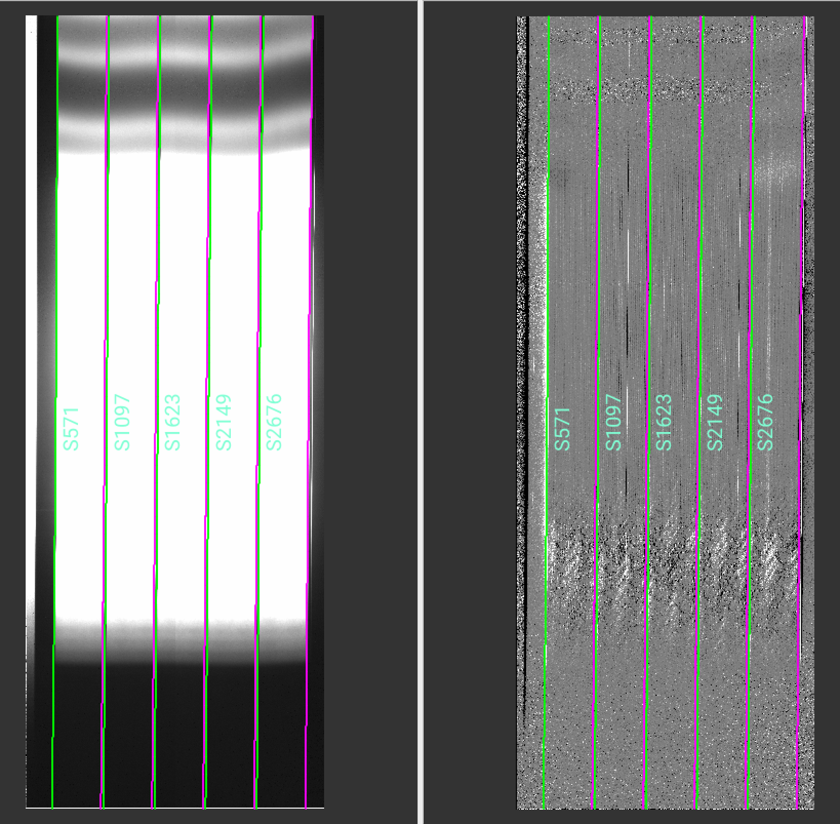
Use the pypeit_chk_edges script (Edges) to confirm that the edges of the slits were correctly traced and that all of the slits were found and that there are no extra slits such as might be produced by pinholes or artifacts of the earlier stages of reduction.
For the segmented science slit, all 5 segments are identified as slits, although only those indicated by slitspatnum will be analyzed.
As an example, for MODS1B,
pypeit_chk_edges Calibrations/Edges_A_0_DET01.fits.gz
will generate an image like the one shown below, where the left and right panels display the slit flat and Sobel filtered image used to detect edges:
Wavelengths
To check the quality of the wavelength calibration, open the Arc_1dfit file in the QA/PNGs subdirectories (in this example, QA/PNGs/Arc_1dfit_A_0_DET01_S1623.png) to insure that the lines have been identified and the RMS is low, ideally < 0.1 pixel, or run pypeit_chk_wavecalib.
pypeit_chk_wavecalib Calibrations/WaveCalib_A_0_DET01.fits
[INFO]    :: Loading WaveCalib from /Users/olga/Library/CloudStorage/Dropbox/Data/MODS_Sample_Datasets/pypeit_rdx/MODS_LS_rdx/lbt_mods1b_proc_A/Calibrations/WaveCalib_A_0_DET01.fits

 N. SpatOrderID minWave Wave_cen maxWave dWave Nlin     IDs_Wave_range    IDs_Wave_cov(%) measured_fwhm  RMS
--- ----------- ------- -------- ------- ----- ---- --------------------- --------------- ------------- -----
  0         571     0.0      0.0     0.0 0.000    0     0.000 -     0.000             0.0           0.0 0.000
  1        1097     0.0      0.0     0.0 0.000    0     0.000 -     0.000             0.0           0.0 0.000
  2        1623  2323.1   4407.5  6506.1 0.516   84  3555.321 -  6404.018            68.1           4.6 0.351
  3        2149     0.0      0.0     0.0 0.000    0     0.000 -     0.000             0.0           0.0 0.000
  4        2676     0.0      0.0     0.0 0.000    0     0.000 -     0.000             0.0           0.0 0.000
The wavelength fit used the combination of the 3 arc images, and was based on the identification of 84 lines. A relatively high RMS ~ 0.35 is not uncommon for MODS Blue. The RMS is improved if just one or two arcs are used, e.g. if only the Argon lamp spectrum is used, the 35 lines still cover the same wavelength range but the fit has an RMS ~ 0.08 pix. The final results do not appear different and using all 3 spectra is still recommended.
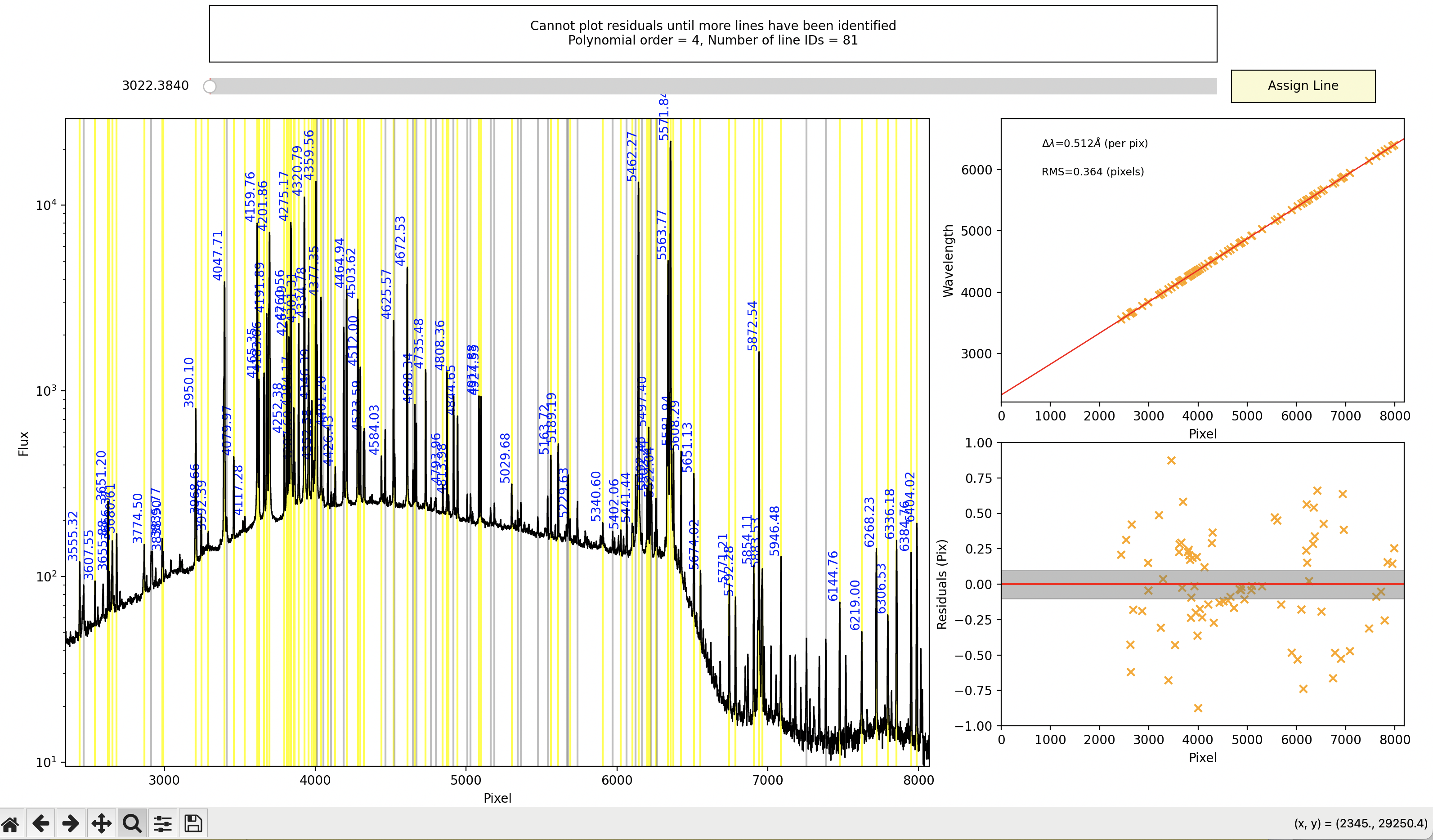
You may refine the wavelength calibration using pypeit_identify. The command below uses the solution found in the pypeit run as a starting point (-s) and uses only slit number 2.
pypeit_identify Calibrations/Arc_A_0_DET01.fits Calibrations/Slits_A_0_DET01.fits.gz -s --slits 2
This plots the arc spectrum and labels all identified lines. Grey lines indicate those lines detected but not identified. How to mark new lines, delete lines and increase or decrease the fit order are all described in pypeit_identify.
Important
Remember, the default calibration is in vacuum wavelengths. The line lists provided on the LBTO Sciops MODS webpages, which contain air wavelengths for lines positively identified in MODS comparison lamp spectra, have been regenerated from NIST in vacuum wavelengths and are part of the default instrument-specific parameters for the lbt_mods#c and lbt_mods#c_proc classes in pypeit.
Spectra
The code will generate 2D and 1D spectra outputs. One per science frame, located in the Science/ folder.
2D spectra
One can inspect the two dimensional spectra
with pypeit_show_2dspec.
It is sometimes helpful to include the -showmask and -removetrace options to display the mask and enable a better view of the residuals around the object. The mask values are explained in Output Bitmasks.
pypeit_show_2dspec Science/spec2d_mods1b.20230909.0028_otf-HS1946+7658_MODS1B_20230909T101314.909.fits
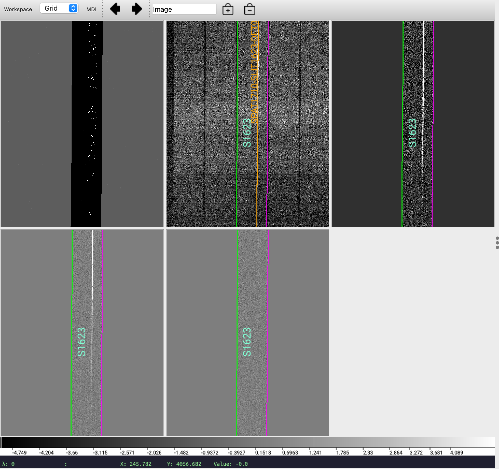
The mask is displayed first (upper left), and then from upper left to lower right are the processed raw image, the sky-subtracted image, the sky-subtracted residuals and the residuals with both sky and object profile subtracted. The spec2D files contain more than 4 extensions. These are listed in the header and can be displayed with ds9 -memf spec2d*fits.
EXT0001 = 'DET01-SCIIMG'
EXT0002 = 'DET01-IVARRAW'
EXT0003 = 'DET01-SKYMODEL'
EXT0004 = 'DET01-OBJMODEL'
EXT0005 = 'DET01-IVARMODEL'
EXT0006 = 'DET01-TILTS'
EXT0007 = 'DET01-SCALEIMG'
EXT0008 = 'DET01-WAVEIMG'
EXT0009 = 'DET01-BPMMASK'
EXT0010 = 'DET01-SLITS'
EXT0011 = 'DET01-WAVESOL'
EXT0012 = 'DET01-SCI_SPEC_FLEXURE'
EXT0013 = 'DET01-MED_CHIS'
EXT0014 = 'DET01-STD_CHIS'
EXT0015 = 'DET01-DETECTOR'
1D spectra
One can inspect the one dimensional spectra with pypeit_show_1dspec, e.g.
pypeit_show_1dspec Science/spec1d_mods1b.20230909.0028_otf-HS1946+7658_MODS1B_20230909T101314.909.fits --ginga
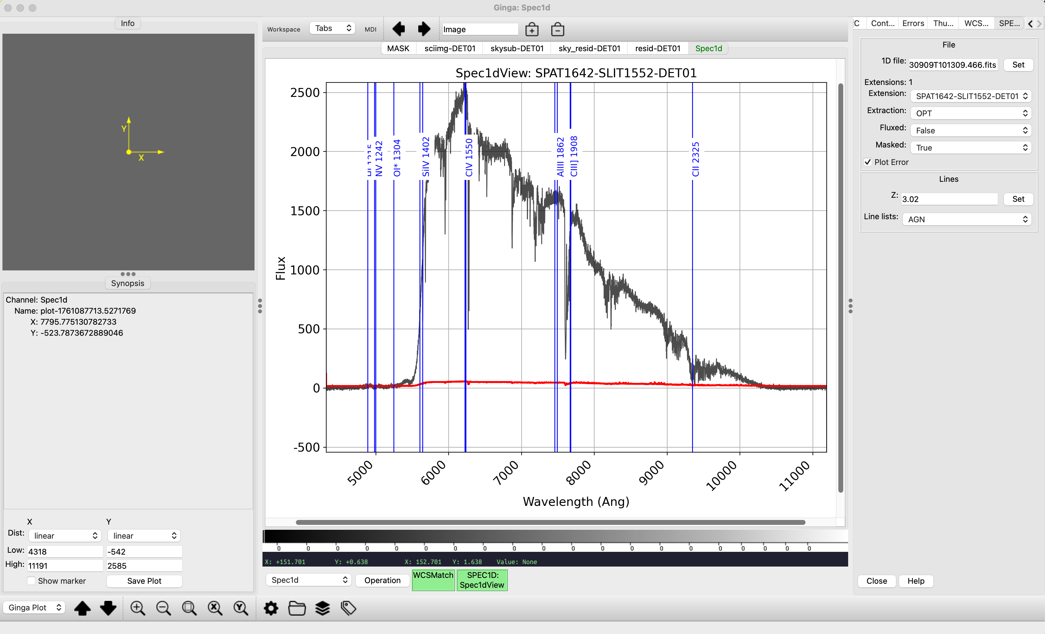
or with a custom python script run within your pypeit environment. For example, the code below will plot the boxcar and optimally extracted spectra for the first object (spec[0]) in the 1D spec file, spec1dfits.
#!/usr/bin/env python

from pypeit import specobjs
import matplotlib.pyplot as plt

spec = specobjs.SpecObjs.from_fitsfile(spec1dfits)
plt.plot(spec[0]['BOX_WAVE'],spec[0]['BOX_COUNTS'])
plt.plot(spec[0]['OPT_WAVE'],spec[0]['OPT_COUNTS'])
Spectral Flexure
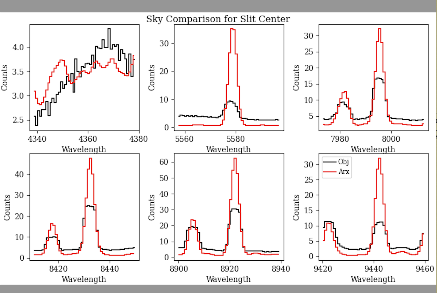
PypeIt performs spectral flexure correction on science targets, although it does not do this for standard stars. The shift is determined by cross-correlating a template sky spectrum which has been convolved with a Gaussian with the FWHM of the arc files with the data. There is both a global correction, applied to all slits, and local correction, an offset from the global one, for each slit. Since most MODS spectra are not taken through the 0.6” slit that is used for the arcs, the procedure may not be exactly correct, but it works well nevertheless. View the set of spec_flex images in QA/PNGs to verify that the flexure correction looks good. For MODS1R, the global spec_flex_sky PNG looks like this:
Flux Calibration
Sensitivity function
As described in Fluxing, pypeit currently has two algorithms to determine the sensitivity function – UVIS for wavelengths < 7000 \(\mathrm{\mathring{A}}\) and IR for spectra at longer wavelengths. The IR method does not apply extinction but does a detailed fitting of the telluric absorption. To maximize the matching of blue and red channel dual grating spectra, it is recommended to use the same algorithm, and the UVIS algorithm works well although some iteration over parameters may be necessary, particularly in the red where, with the UVIS algorithm, it is necessary to fit across regions of telluric absorption. Overriding the default resolution with the resolution of MODS (R~2000, 0.6” slit), setting the breakpoint spacing to 40 rather than the default 20 times the resolution element, and using a fairly low order may help, but if the order is too low, then the wiggles in the dichroic transmission may be washed out.
The script pypeit_sensfunc generates the sensitivity function from a single spectrophotometric standard star spectrum. Since MODS scripts typically take 3 back-to-back standard star integrations, it can be reassuring to overplot these (you may need to write a custom script with commands similar to those shown above) to insure that there was no significant variation between them and to select the best. pypeit_sensfunc reads in a sensfunc input file and the filename of the 1D spectrum to use. For this dataset, the commands were the following, and the input files are shown below:
pypeit_sensfunc -s mods1b_dual.sens Science/spec1d_mods1b.20230909.0024_otf-Feige110dualgrating_MODS1B_20230909T084730.480.fits --debug -v 2
and
pypeit_sensfunc -s mods1r_dual.sens Science/spec1d_mods1r.20230909.0044_otf-Feige110dualgrating_MODS1R_20230909T084726.333.fits --debug -v 2
The debug and high verbosity (v = [0,1,2]) options are helpful, especially when starting to reduce a dataset.
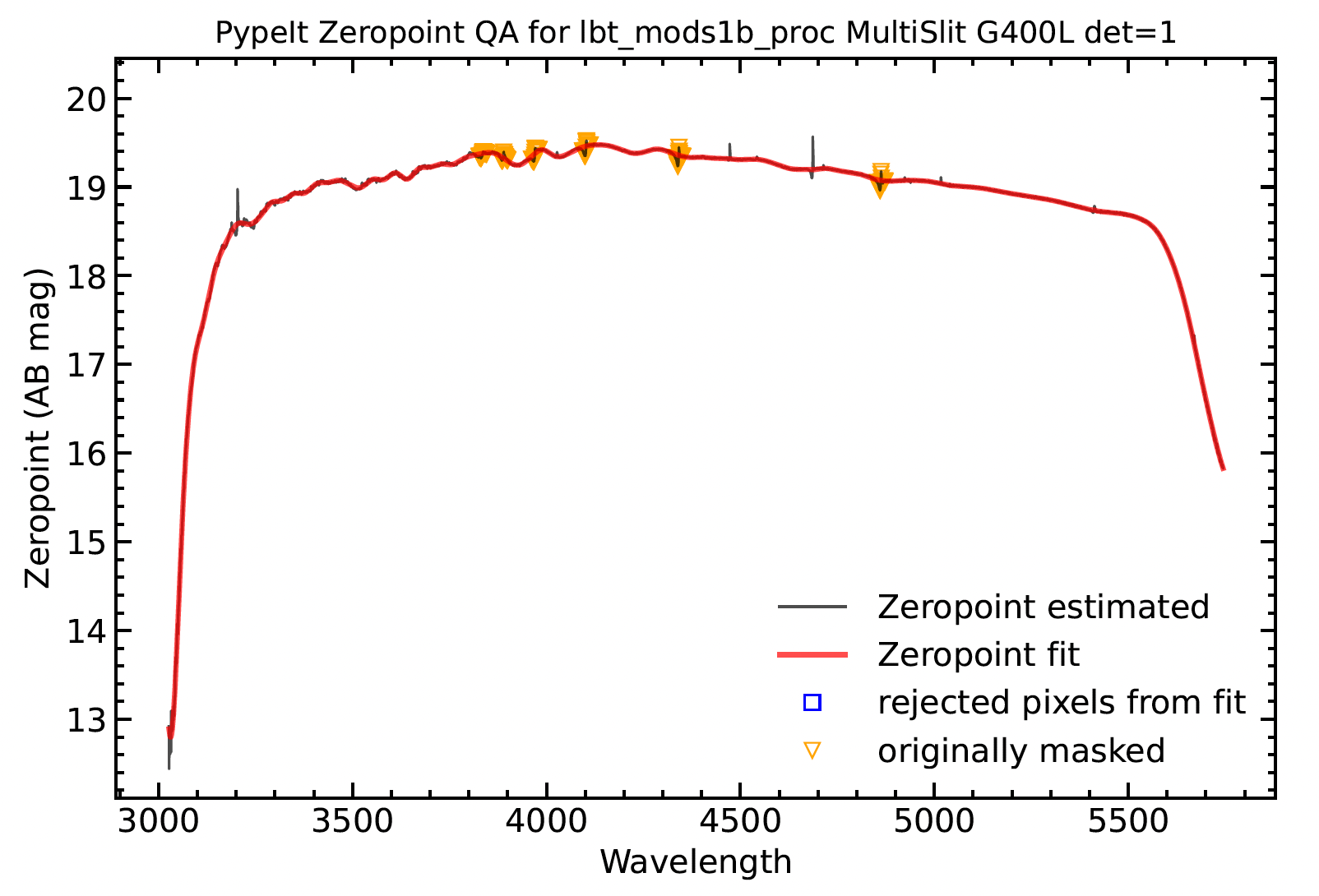
pypeit_sensfunc outputs the sensitivity function as a fits file and also 3 PDFs: one of the throughput vs wavelength; another of the zeropoint vs wavelength; and a third of the flux-calibrated standard star spectrum, with the tabulated spectrum overplotted in green for comparison.
Note
Note that the proc classes do not apply the CCD conversion gain, so the sensitivity functions generated for these will differ from those generated for the original mods classes, but so long as the use is consistent there will be no problem.
Note
Note that pypeit uses spectroscopic zeropoints, which are defined so that a source with a flat spectrum in frequency and an AB magnitude equal to the zeropoint will produce 1 photon/s/\(\mathrm{\mathring{A}}\) on the detector. To convert these zeropoints (\(ZP\)) to the zeropoints tabulated on the LBTO Sciops MODS webpages (\(ZP_m\)):
\(ZP_m\) = 0.4 \(ZP\) + 2 log10(\(\lambda\)) + 0.964 - log10(g)
where \(\lambda\) is the wavelength in \(\mathrm{\mathring{A}}\) and g, the conversion gain in e-/ADU (g=1 for the proc classes).
Sample sensfunc input files for the blue and red channels are given below.
Blue
For the blue channel, mods1b_dual.sens is:
[sensfunc]
   algorithm = UVIS
   extr = OPT
   polyorder = 25 # default is 7, higher order to fit wiggles in dichroic transmission
   extrap_blu = 0.3
   extrap_red = 0.15
   trim_std_pixs = 1400,1500 #for MODS1B Dual Grating, 3027-5745 Angstroms
   use_flat = False
   # for algorithm = UVIS
   [[UVIS]]
      extinct_correct = True
      extinct_file = lbtoextinct.dat
The dual grating standard star spectrum drops precipitously in the blue, at the atmospheric cutoff, and in the red, due to the dichroic transmission. For this reason, trim_std_pixs was set to trim the first 1400 and the last 1500 pixels. These values were determined by locating the wavelength of the sharp turndown on the 1D spectrum plot and then reading off the corresponding pixel value on the 2D spectrum plot. The extrap_blu and extrap_red were set to extrapolate the fit to endpoints of the spectral range.
The polyorder has been increased over the default to fit through wiggles in the dichroic transmission function.
Hydrogen absorption lines are masked, and the default 10 \(\mathrm{\mathring{A}}\) setting appears to be fine. Uncorrected flexure causes ‘P-Cygni’-like profiles for the hydrogen lines, but because these are masked, the fit is unaffected. But there is an absorption line, probably HeII/5411 angstroms, in some standards (e.g. Feige 110) which is not masked and contributes a small-scale blip in the sensitivity function.
Red
For the red channel, mods1r_dual.sens is:
[sensfunc]
  algorithm = UVIS

  extr = OPT
  polyorder = 6

  hydrogen_mask_wid = 15. #default is 10.
  trim_std_pixs = 1600,1100  #for MODS1R Dual Grating 5635 - 10272 angstroms

  extrap_blu = 0.4
  extrap_red = 0.1

  use_flat = False


  # for algorithm = UVIS
  [[UVIS]]
     nresln = 40 # default is 20
     resolution = 2000 # default is 3000
     extinct_correct = True
     extinct_file = lbtoextinct.dat
     telluric = True
     telluric_correct = True
     trans_thresh = 0.97 # default is 0.9
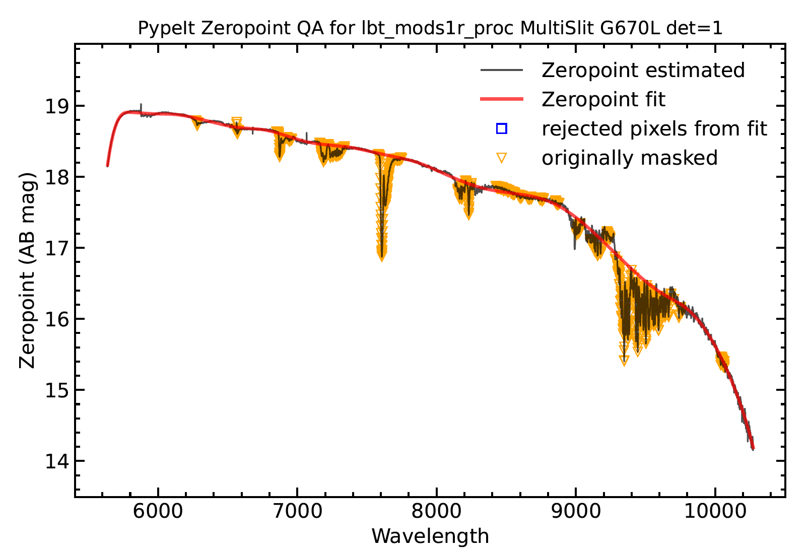
The zeropoints vs wavelength PDF is shown below.
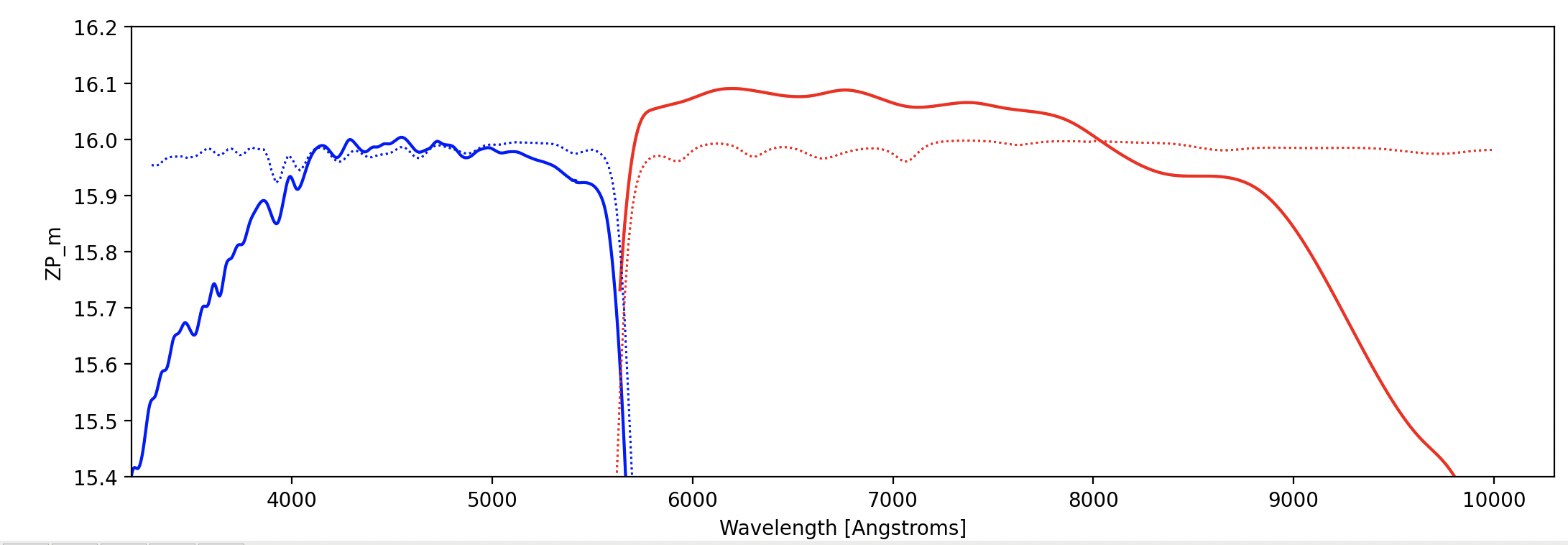
To illustrate that the fits to the sensitivity function account for the wiggles in the dichroic transmission curves, the MODS1 Dual Red and Dual Blue zeropoint fits output by pypeit_sensfunc (solid blue or red curves) are plotted together with the MODS1 dichroic transmission curves which have been scaled to overlap (dotted), below.
Flux Calibrating the spectra
Setup files for the next three steps: flux calibrating the spectra, coadding these, and correcting for telluric absorption; are generated with a single script, pypeit_flux_setup.
Flux Calibration
First the spectra are flux calibrated, using the sensitivity functions just generated. The following commands were used, and the input flux files are included below.
pypeit_flux_calib lbt_mods1b_proc.flux
and
pypeit_flux_calib lbt_mods1r_proc.flux
lbt_mods1b_proc.flux:
# Auto-generated Flux input file using PypeIt version: 1.18.0
# UTC 2025-10-18T19:37:47.788+00:00

# User-defined execution parameters
[fluxcalib]
  extinct_correct = True # Set to True if your SENSFUNC derived with the UVIS algorithm
# Please add your SENSFUNC file name below before running pypeit_flux_calib

# Data block
flux read
 path Science
 path .
                                                                           filename |                                                                          sensfile
spec1d_mods1b.20230909.0024_otf-Feige110dualgrating_MODS1B_20230909T084730.480.fits | sens_mods1b.20230909.0024_otf-Feige110dualgrating_MODS1B_20230909T084730.480.fits
        spec1d_mods1b.20230909.0028_otf-HS1946+7658_MODS1B_20230909T101314.909.fits |
flux end
lbt_mods1r_proc.flux:
# Auto-generated Flux input file using PypeIt version: 1.18.0
# UTC 2025-10-18T19:56:18.092+00:00

# User-defined execution parameters
[fluxcalib]
  extinct_correct = True  # Set to True if your SENSFUNC derived with the UVIS algorithm
# Please add your SENSFUNC file name below before running pypeit_flux_calib

# Data block
flux read
 path Science
 path .
                                                                           filename |                                                                          sensfile
        spec1d_mods1r.20230909.0051_otf-HS1946+7658_MODS1R_20230909T101309.466.fits | sens_mods1r.20230909.0044_otf-Feige110dualgrating_MODS1R_20230909T084726.333.fits
spec1d_mods1r.20230909.0044_otf-Feige110dualgrating_MODS1R_20230909T084726.333.fits |
Coadding the 1D spectra
Next, the individual flux-calibrated spectra may be coadded using the script pypeit_coadd_1dspec script. Parameter values to override the defaults are added to the input file. there are several options for handling the differences in the wavelength arrays, which result for several reasons: each spectrum may have been individually wavelength calibrated, if the OH lines are used as in the near-infrared; individually corrected for spectral flexure; or extracted from a different position along the slit, if dithering has been done; and when wave_method is set to linear or velocity, the output spectrum is linearized to the constant dispersion that is specified by dwave or dvel.
Note
The datamodel for the output of pypeit_coadd_1dspec script is different from that for the 1D specra output by run_pypeit, and it is the one required for telluric correction by pypeit_tellfit; therefore, before correcting for telluric absorption, it is necessary to run pypeit_coadd_1dspec even if you have only a single target spectrum.
pypeit_coadd_1dspec lbt_mods1b_proc.coadd1d --debug -v 2 --show
and
pypeit_coadd_1dspec lbt_mods1r_proc.coadd1d --debug -v 2 --show
The input files, lbt_mods1b_proc.coadd1d and lbt_mods1r_proc.coadd1d (see below), have wave_method, dwave, wave_grid_min and wave_grid_max all specified, in order to output blue and red spectra with the same dispersion and to cut off the endpoints which are noisy. The value, dwave = 0.85 \(\mathrm{\mathring{A}}\), was chosen simply because it is larger of the blue and red channel linear dispersions.
lbt_mods1b_proc.coadd1d:
# Auto-generated Coadd1D input file using PypeIt version: 1.18.0
# UTC 2025-10-18T19:37:47.795+00:00

# User-defined execution parameters
[coadd1d]
  coaddfile = m1b_HS1946+7658_coadd1d.fits # Please set your output file name
  wave_method = linear  # creates a uniformly space grid in lambda
  dwave = 0.85
  wave_grid_min = 3400
  wave_grid_max = 5700
# This file includes all extracted objects. You need to figure out which object you want to
# coadd before running pypeit_coadd_1dspec!!!

# Data block
coadd1d read
 path Science
 path .
                                                                           filename |                  obj_id
        spec1d_mods1b.20230909.0028_otf-HS1946+7658_MODS1B_20230909T101314.909.fits | SPAT1710-SLIT1623-DET01
coadd1d end
lbt_mods1r_proc.coadd1d:
# Auto-generated Coadd1D input file using PypeIt version: 1.18.0
# UTC 2025-10-18T19:56:18.097+00:00

# User-defined execution parameters
[coadd1d]
  coaddfile = m1r_HS1946+7658_coadd1d.fits  # Please set your output file name
  wave_method = linear  # creates a uniformly space grid in lambda
  dwave = 0.85
  wave_grid_min = 5500
  wave_grid_max = 10270
# This file includes all extracted objects. You need to figure out which object you want to
# coadd before running pypeit_coadd_1dspec!!!

# Data block
coadd1d read
 path Science
 path .
                                                                           filename |                  obj_id
        spec1d_mods1r.20230909.0051_otf-HS1946+7658_MODS1R_20230909T101309.466.fits | SPAT1642-SLIT1552-DET01
coadd1d end
Correcting the Telluric Absorption
Under construction…